Introduction
In previous reference material, governing principles of fluid mechanics were developed using conservation of mass, momentum, and energy. Many practical engineering systems apply these principles to flows moving through enclosed passages such as pipes, tubes, ducts, and channels.
Pipe flow is important in a wide range of applications including water distribution systems, HVAC systems, hydraulic machinery, oil and gas transport,cooling systems, and more. Although the geometry of a pipe may appear simple, the resulting flow behavior can vary significantly depending on the effects of viscosity, pressure gradients, pipe roughness, and flow speed.
Unlike certain inviscid flow models used in earlier chapters, viscous effects in pipe flow are often dominant and directly influence the pressure losses required to maintain fluid motion. Energy supplied by pumps or elevation differences is continually dissipated through viscous shear within the fluid and at the pipe walls. This chapter focuses on the behavior of incompressible viscous flow in pipes. Important topics include laminar and turbulent flow behavior, entrance region development, pressure losses, velocity profiles, friction factors, and pipe system analysis. Both major losses associated with wall friction and minor losses associated with components such as valves, bends, and fittings are considered as well.
Engineers will find this information useful in analyzing the performance of pipe systems as well as sizing components like pumps or air conditioners to achieve a particular thermo-fluidic output.
Basic Theory of Pipe Flow
Pipe flow refers to fluid motion through enclosed passages that are completely filled with fluid. This is contrasted with what is commonly termed open-channel flow in which the fluid conduit is only partially occupied with fluid with the rest being exposed to ambient conditions such as in a gutter. It should be noted that the mechanics of open-channel flow are different from pipe flow.
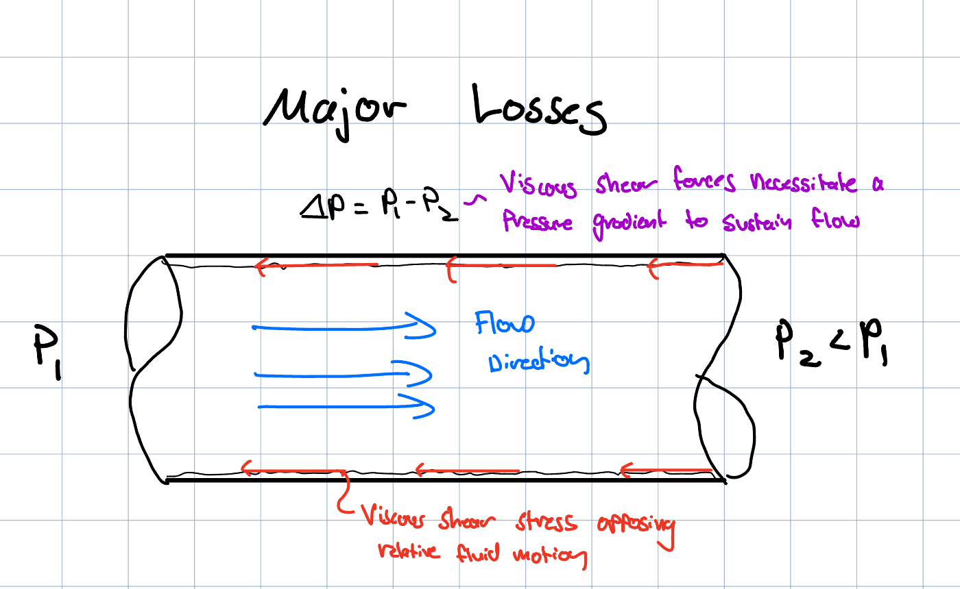
An important and often defining feature of pipe flow is that fluid motion is usually driven by a pressure difference or gradient along a length of pipe. As the fluid moves downstream, viscous effects at the wall create shear stresses that resist the motion of the fluid. This resistance produces pressure losses and converts mechanical energy into thermal energy through viscous dissipation. In this way pipe flow represents an interaction between pressure gradients and viscous forces that define the velocity profile and flow characteristics inside of the pipe conduit.
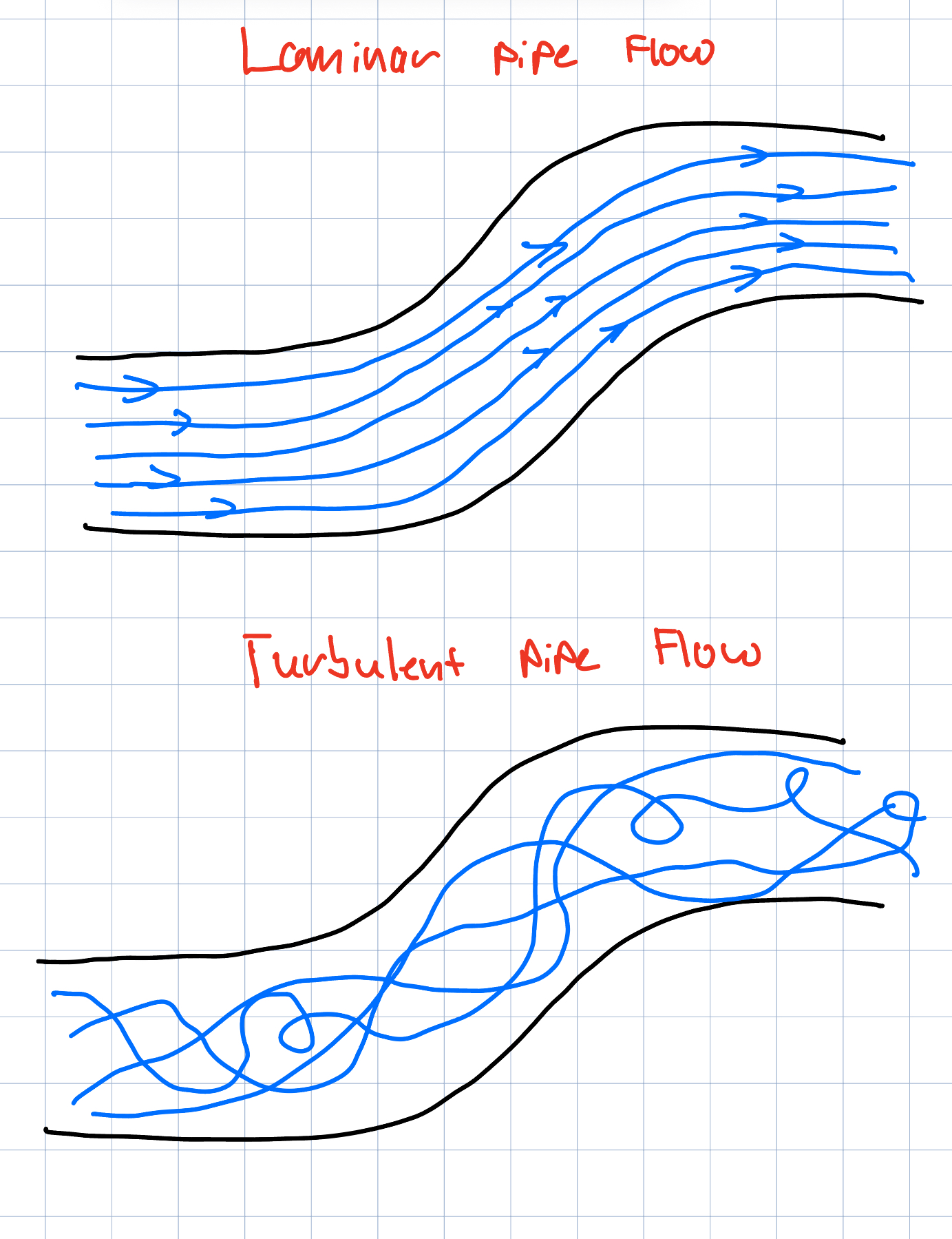
Laminar and Turbulent Flow
Pipe flow may be classified as laminar, transitional, or turbulent. For laminar flow, fluid particles move in relatively smooth layers with limited mixing between neighboring fluid elements. In turbulent flow, velocity and pressure fluctuate continuously and strong mixing occurs throughout the flow. Transitional flow occupies an intermediate state, where smooth flow characeristics are unstable or sporadically interrupted by turbulent mixing. Perhaps unsurprisingly, whether a flow displays laminar or turbulent characteristics depends primarily on the Reynolds number. Indeed, viscous forces are dominant in laminar flow whereas inertial forces are more significant in turbulent flow. For pipe flow, the Reynolds number is given as:- \( \rho \) is fluid density,
- \( V \) is average velocity,
- \( D \) is pipe diameter,
- \( \mu \) is dynamic viscosity.
Defining fully developed flow
When fluid first enters a pipe, the velocity profile is often nearly uniform. Due to the no-slip condition, fluid near the wall slows down and boundary layers (boundary layers are covered in greater detail in Chapter 9; in pipe flow this is a region where viscous effects are relevant to the flow) begin growing inward from the pipe surface.
As the flow continues downstream, the boundary layers increase in thickness until they merge at the pipe centerline. Beyond this point, the velocity profile no longer changes shape in the flow direction and the flow is said to be fully developed. The distance required for the flow to become fully developed is called the entrance length.The final shape of the flow profile as well as the entrance length depends on the nature of the incoming flow, be it laminar or turbulent. For laminar flow, the entrance length is approximately:
Pressure gradients: The drivers of pipe flow
For fully developed flow in a horizontal pipe, pressure decreases in the flow direction because energy is continually lost due to viscous shear at the wall: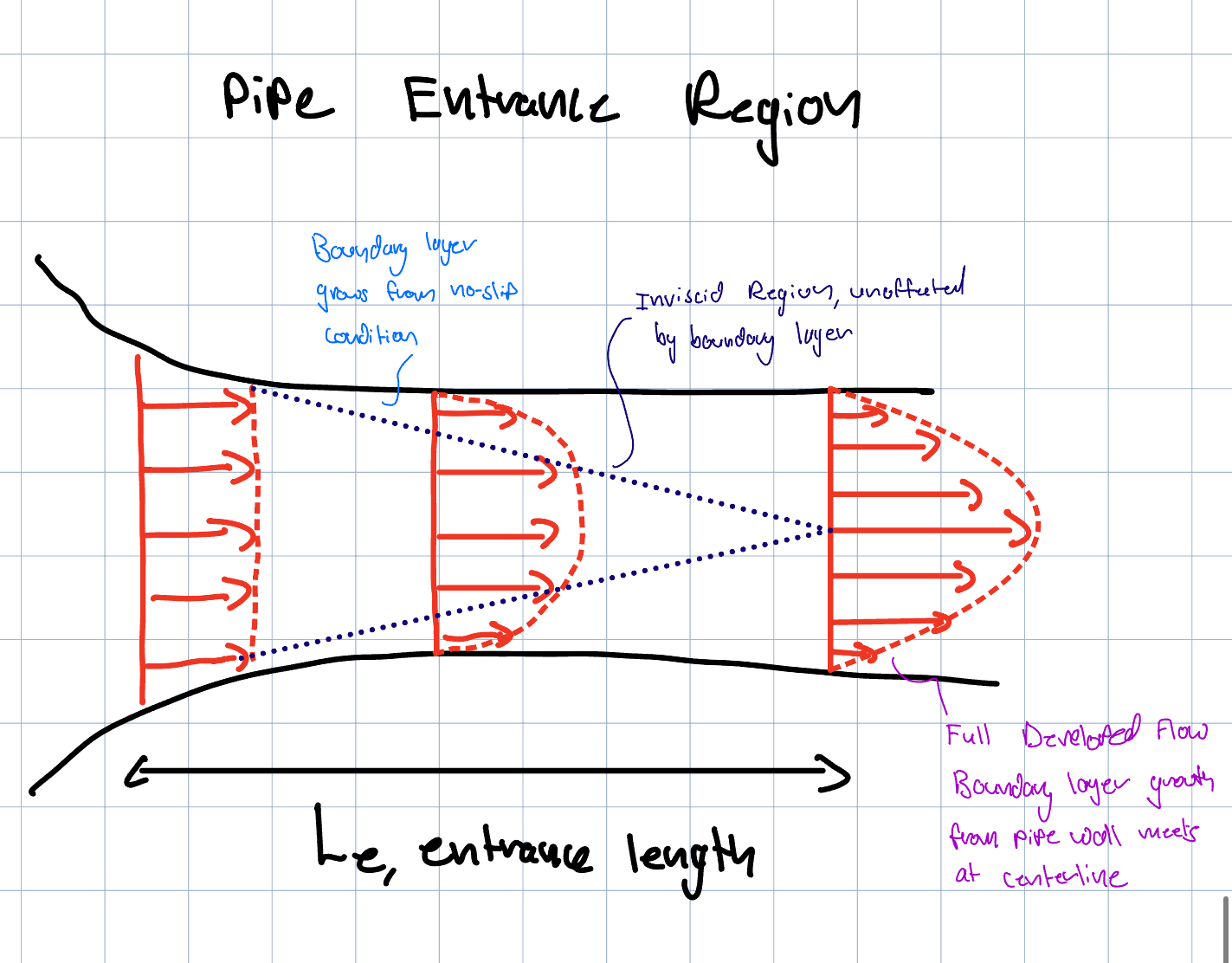
Developed Laminar Flow
For sufficiently small Reynolds numbers, pipe flow remains laminar and fluid motion occurs in relatively smooth layers with limited mixing between adjacent fluid particles. After the entrance region ends, the velocity profile no longer changes shape in the flow direction and the flow becomes fully developed.
For steady, incompressible, fully developed flow in a horizontal circular pipe, the axial velocity depends only on radial position:
Velocity Distribution
Applying the momentum equation together with Newton's law of viscosity leads to the classical laminar pipe velocity profile:- \( R \) is the pipe radius,
- \( r \) is the radial coordinate,
- \( \Delta p \) is the pressure drop across pipe length \( L \).
Pressure Drop and Wall Shear Stress
Take note from the preceding equations that the pressure drop required to maintain flow increases with:- increasing flow rate,
- increasing viscosity,
- increasing pipe length,
Darcy Friction Factor
Pressure losses in pipe flow are commonly modeled using the Darcy friction factor:Fully Developed Turbulent Pipe Flow
At sufficiently large Reynolds numbers, pipe flow becomes turbulent and the fluid motion contains strong velocity fluctuations and mixing throughout the flow. Unlike laminar flow, turbulent motion continuously transfers momentum between different fluid regions, producing larger wall shear stresses and greater pressure losses.
As with laminar flow, turbulent pipe flow eventually becomes fully developed after the entrance region. In fully developed turbulent flow, the average velocity profile no longer changes shape in the flow direction, although instantaneous velocity fluctuations still occur.
Velocity Profile
Turbulent mixing causes momentum to be transported more effectively across the pipe cross section than in laminar flow. As a result, the turbulent velocity profile is generally flatter through most of the pipe interior with steep velocity gradients near the wall.
Unlike laminar flow, there is no simple exact analytical solution for the full turbulent velocity distribution. However, approximate empirical profiles are commonly used. One common approximation is the power-law profile:
- \( u \) is the local velocity,
- \( u_{\max} \) is the centerline velocity,
- \( R \) is the pipe radius,
- \( n \) is an experimentally determined exponent.
Pressure Losses
Pressure losses in turbulent pipe flow are substantially larger than in laminar flow because of increased momentum mixing and wall shear stress. The pressure drop is commonly expressed using the Darcy--Weisbach equation:- \( f \) is the Darcy friction factor,
- \( L \) is pipe length,
- \( D \) is pipe diameter,
- \( V \) is average velocity.
Friction Factor Behavior
Unlike laminar flow, the turbulent friction factor depends on both Reynolds number and pipe roughness:Energy Dissipation in Turbulent Flow
Turbulent pipe flow produces greater energy dissipation than laminar flow because eddies and continuous chatoic swirling continually transfers momentum and kinetic energy throughout the fluid, prompting greater losses due to friction or viscosity. As Reynolds number increases, turbulent mixing generally becomes stronger, leading to larger pressure losses and usually greater pumping power requirements.Pipe Flow Losses
As fluid moves through a pipe system, mechanical energy is continually lost due to viscous effects. These losses appear primarily as pressure drops and must often be overcome using pumps, fans, or elevation differences. Pipe flow losses are commonly divided into two categories:- major losses,
- minor losses.
Major Losses
Major losses are associated with viscous friction along the walls of a pipe. These losses accumulate continuously over the pipe length and are usually the dominant source of pressure drop in long pipe systems.
The pressure loss due to wall friction is commonly modeled using the Darcy--Weisbach equation:
- \( f \) is the Darcy friction factor,
- \( L \) is pipe length,
- \( D \) is pipe diameter,
- \( V \) is average velocity.
Moody Chart
As already stated above, for turbulent pipe flow, the Darcy friction factor depends on both Reynolds number and relative roughness:- \( \epsilon \) is the average roughness height,
- \( D \) is the pipe diameter.
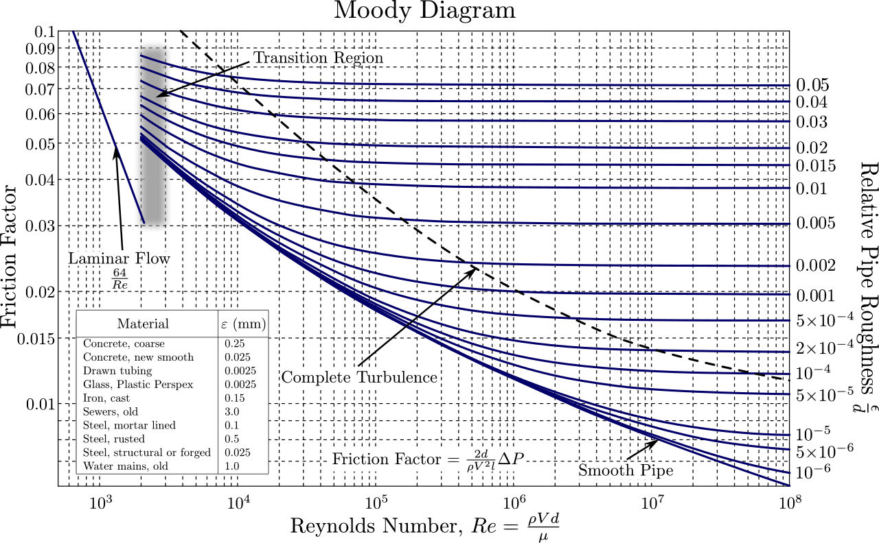
- Compute the Reynolds number:
- Determine the pipe relative roughness:
- Locate the Reynolds number on the horizontal axis.
- Move vertically until intersecting the appropriate relative roughness curve.
- Read the Darcy friction factor from the vertical axis.
- The friction factor can then be used to estimate major losses in a pipe system
Colebrook Equation
When working with the Moody diagram and major losses, an engineer might hear of the Colebrook formula. The Colebrook equation provides an implicit relationship for the Darcy friction factor in turbulent pipe flow:- \( f \) is the Darcy friction factor,
- \( Re \) is the Reynolds number,
- \( \epsilon \) is the pipe roughness,
- \( D \) is the pipe diameter.
Minor Losses
Minor losses arise from localized disturbances to the flow caused by components such as:- bends,
- valves,
- fittings,
- entrances and exits,
- contractions and expansions.
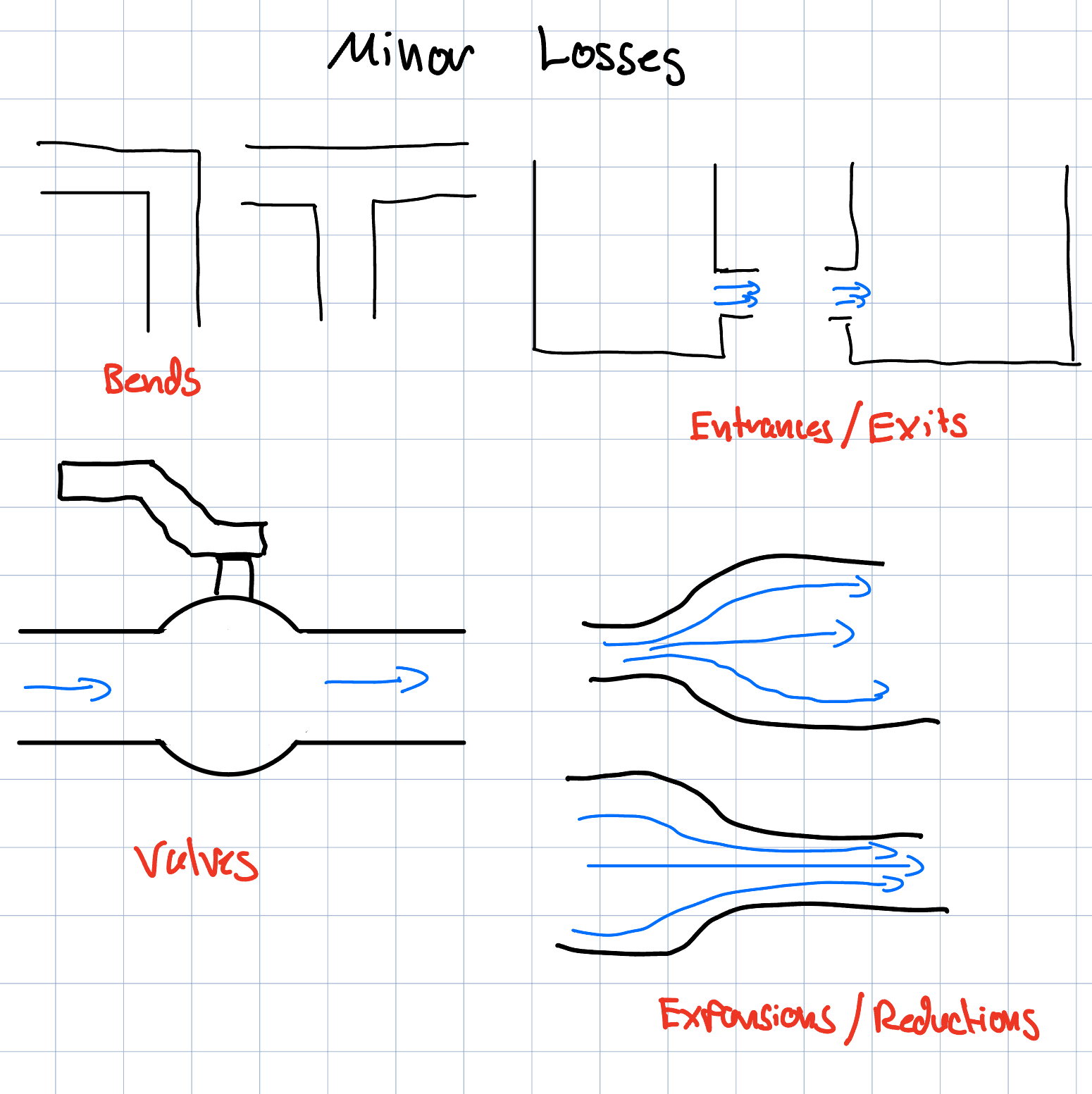
| Component | Typical \( K \) Value |
|---|---|
| Sharp-edged entrance | 0.5 |
| Well-rounded entrance | 0.04 |
| Pipe exit | 1.0 |
| Standard 90\( ^\circ \) elbow | 0.3 -- 1.5 |
| 45\( ^\circ \) elbow | 0.2 -- 0.4 |
| Fully open gate valve | 0.15 |
| Fully open globe valve | 10 |
| Fully open angle valve | 2 |
| Fully open ball valve | 0.05 |
| Sudden expansion | \( \left(1-\dfrac{A_1}{A_2}\right)^2 \) |
| Sudden contraction | 0.4 -- 1.0 |