Current page:

Plasticity

Ductility
Yield Strength
Ultimate Strength
Failure

Material Properties

Continuum Mechanics Fundamentals

Generally, the state of stress a 3D material can be represented as a second-rank tensor (i.e. a matrix) with $ 3^2 = 9 $ components.

Infinitesimal Stress element

Stress tensor.

$$ \boldsymbol{\sigma} = \begin{bmatrix} \sigma_{11} & \sigma_{12} & \sigma_{13} \\ \sigma_{21} & \sigma_{22} & \sigma_{23} \\ \sigma_{31} & \sigma_{32} & \sigma_{33} \end{bmatrix} \ $$

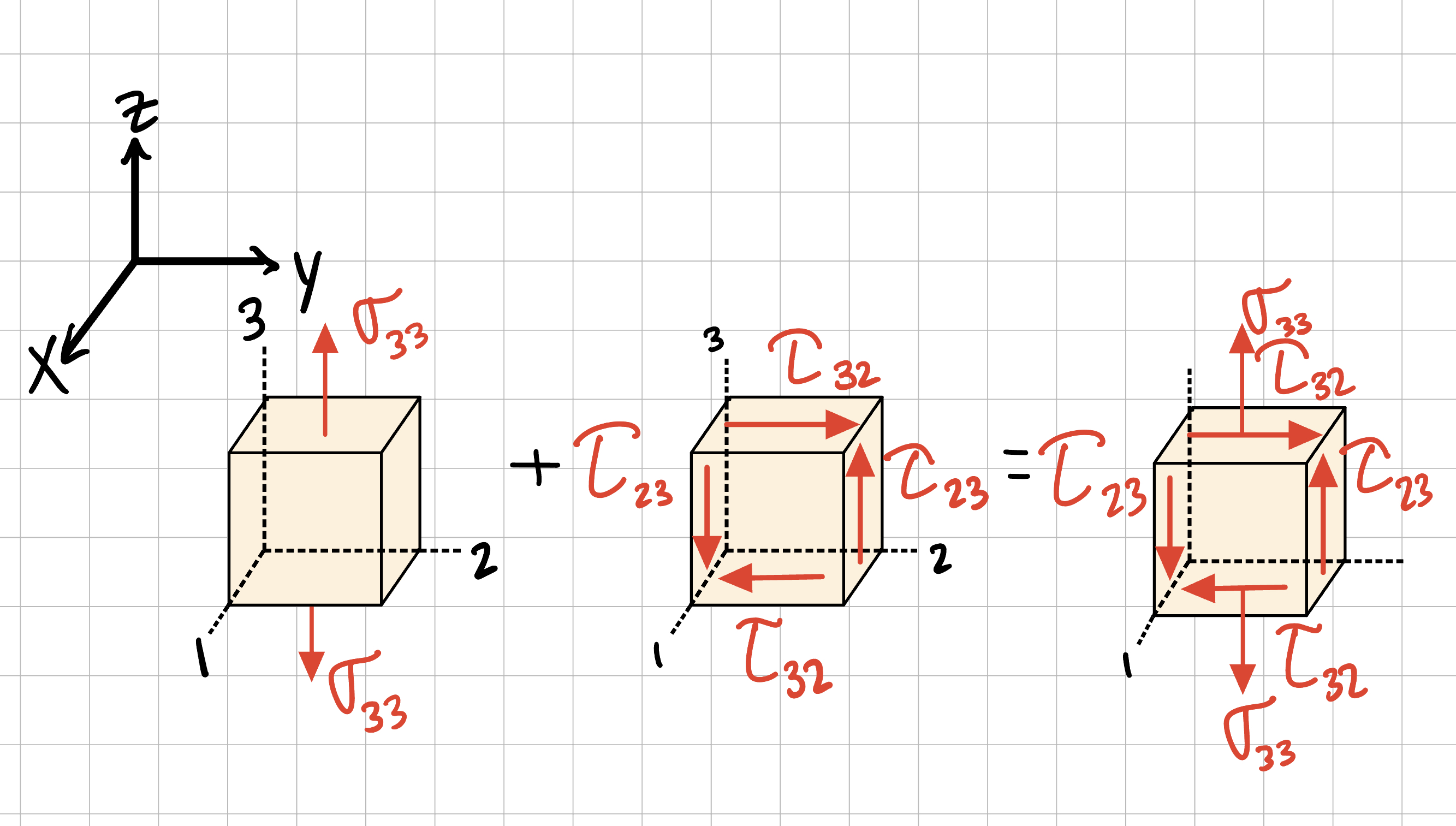
Using indicial notation, component $ (i, j) $ of this tensor is denoted as $ \sigma_{ij} $. The same can be said for a material strain tensor.

Infinitesimal Strain Element

Strain tensor.

$$ \boldsymbol{\varepsilon} = \begin{bmatrix} \varepsilon_{11} & \varepsilon_{12} & \varepsilon_{13} \\ \varepsilon_{21} & \varepsilon_{22} & \varepsilon_{23} \\ \varepsilon_{31} & \varepsilon_{32} & \varepsilon_{33} \end{bmatrix} \ $$

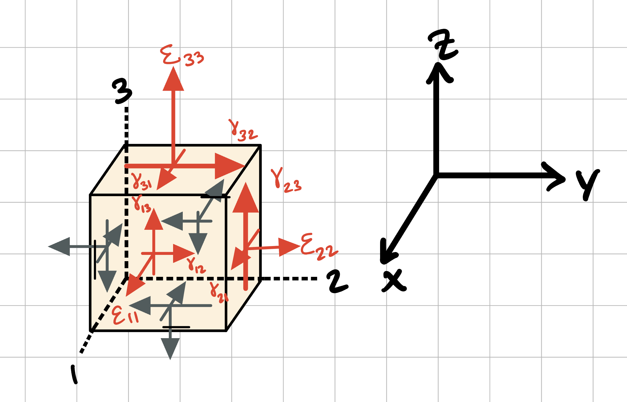
Using indicial notation, component $ (k, l) $ of this tensor is denoted as $ \varepsilon_{kl} $. Note that both the stress and strain tensors are symmetric, that is $ \sigma_{ij} = \sigma_{ji} $ and $ \varepsilon_{kl} = \varepsilon_{lk} $.

For our purposes, lets bound the discussion of material stress-strain behavior to only the elastic range, that is, deformation is linear proportional applied load. This is Hooke’s law. The relationship between stress and strain is referred to as the constitutive relationship of a material. In the most general case, this relationship is defined as a fourth-rank tensor with $ 3^4=81 $ components. This elasticity tensor, C, relating the stress and strain tensors is shown in indicial notation (rather than a matrix operation).

Hooke's law general form. #mat-hls

$$ \sigma_{ij} = C_{ijkl}\varepsilon_{kl} $$

This is short form representation of a summation, known as indicial notation. Whenever there are repeated indices on the right hand side of an equation, as with k and l above (repeated in $ C_{ij\mathbf{kl}} $ and $ \varepsilon_{\mathbf{kl}} $), these indices represent a summation over three dimensions. So the example can be rewritten as shown below, where $ k\ \in \{1 \ 2 \ 3\} $ and $ l\ \in \{1 \ 2 \ 3\} $.

$$ \sigma_{ij} = \sum_{k=1}^{3}\sum_{l=1}^{3}C_{ijkl}\varepsilon_{kl} $$

Expanding over these two summations yields:

$$ \begin{aligned}\sigma_{ij} = &C_{ij11}\varepsilon_{11} + C_{ij12}\varepsilon_{12} + C_{ij13}\varepsilon_{13} \\ + &C_{ij21}\varepsilon_{21} + C_{ij22}\varepsilon_{22} + C_{ij23}\varepsilon_{23} \ + C_{ij31}\varepsilon_{31} + C_{ij32}\varepsilon_{32} + C_{ij33}\varepsilon_{33}\end{aligned} $$

What this means is there can be as many as 9 components of strain and 9 material coefficients that contribute to each stress component. (You can see the benefit of indicial notation here.)

However, not all 81 components of this tensor are independent, because of symmetry of stress and strain tensors there are only 21 independent components. If the material is assumed to be isotropic (having the same behavior in all directions) this is further reduced to just 2 independent components (for instance, $ E $ Young’s modulus and $ \nu $, Poisson’s ratio). With this simplification, the 3D isotropic elastic material constitutive relation can be simplified.

Voigt notation.

$$ \begin{bmatrix} \varepsilon_{11} \\ \varepsilon_{22} \\ \varepsilon_{33} \\ 2\varepsilon_{23} \\ 2\varepsilon_{13} \\ 2\varepsilon_{12} \end{bmatrix} = \begin{bmatrix} \varepsilon_{11} \\ \varepsilon_{22} \\ \varepsilon_{33} \\ \gamma_{23} \\ \gamma_{13} \\ \gamma_{12} \end{bmatrix} = \frac{1}{E} \begin{bmatrix} 1 & -\nu & -\nu & 0 & 0 & 0 \\ -\nu & 1 & -\nu & 0 & 0 & 0 \\ -\nu & -\nu & 1 & 0 & 0 & 0 \\ 0 & 0 & 0 & 2 + 2\nu & 0 & 0 \\ 0 & 0 & 0 & 0 & 2 + 2\nu & 0 \\ 0 & 0 & 0 & 0 & 0 & 2 + 2\nu \end{bmatrix} \begin{bmatrix} \sigma_{11} \\ \sigma_{22} \\ \sigma_{33} \\ \sigma_{23} \\ \sigma_{13} \\ \sigma_{12} \end{bmatrix} $$

Here the engineering shear strains $ \gamma_{23},\gamma_{13},\gamma_{12} $ are introduced. This, along with identification of shear stresses $ \sigma_{23},\sigma_{13},\sigma_{12} $ as $ \tau_{23},\tau_{13},\tau_{12} $ allows for the expression for pure axial stress & strain in one direction to be represented as $ \varepsilon_{11} = \frac{\sigma_{11}}{E} $. Rearranging the terms, relation can be expressed in a more general form.

Simplified Hooke's Law.

$$ \sigma = E\varepsilon $$

Similarly, the expression for pure shear stress & strain can be expressed as $ \gamma_{12} = \frac{\tau_{12}(2+2\nu)}{E} = \frac{\tau_{12}}{G} $. Again, this can be expressed in a more general form.

Simplified shear stress equation.

$$ \tau = \gamma G $$

Extra!

If you want more details on this topic, consider taking a course in continuum mechanics.

Notation Note

Bold symbols, such as $ \boldsymbol{\sigma} $ and $ \boldsymbol{\varepsilon} $, represent tensors rather than scalar quantities.

Additionally, some quantities might be represented with indicial notation. When indices on the right hand side of the equation are repeated, this represents a summation where the index values range from 1 to 3. For example,

$$ \sigma_{ij} = C_{ijkl}\varepsilon_{kl} $$

represents

$$ \sigma_{ij} = \sum_{k=1}^{3}\sum_{l=1}^{3}C_{ijkl}\varepsilon_{kl} $$

This is a shorthand to make writing long summations easier.

Stress-Strain Diagram

Stress-strain diagram showing key properties

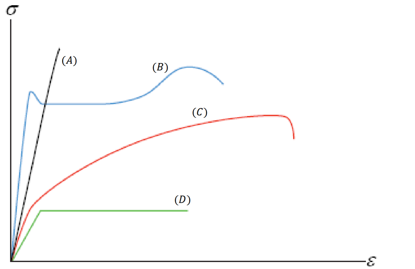
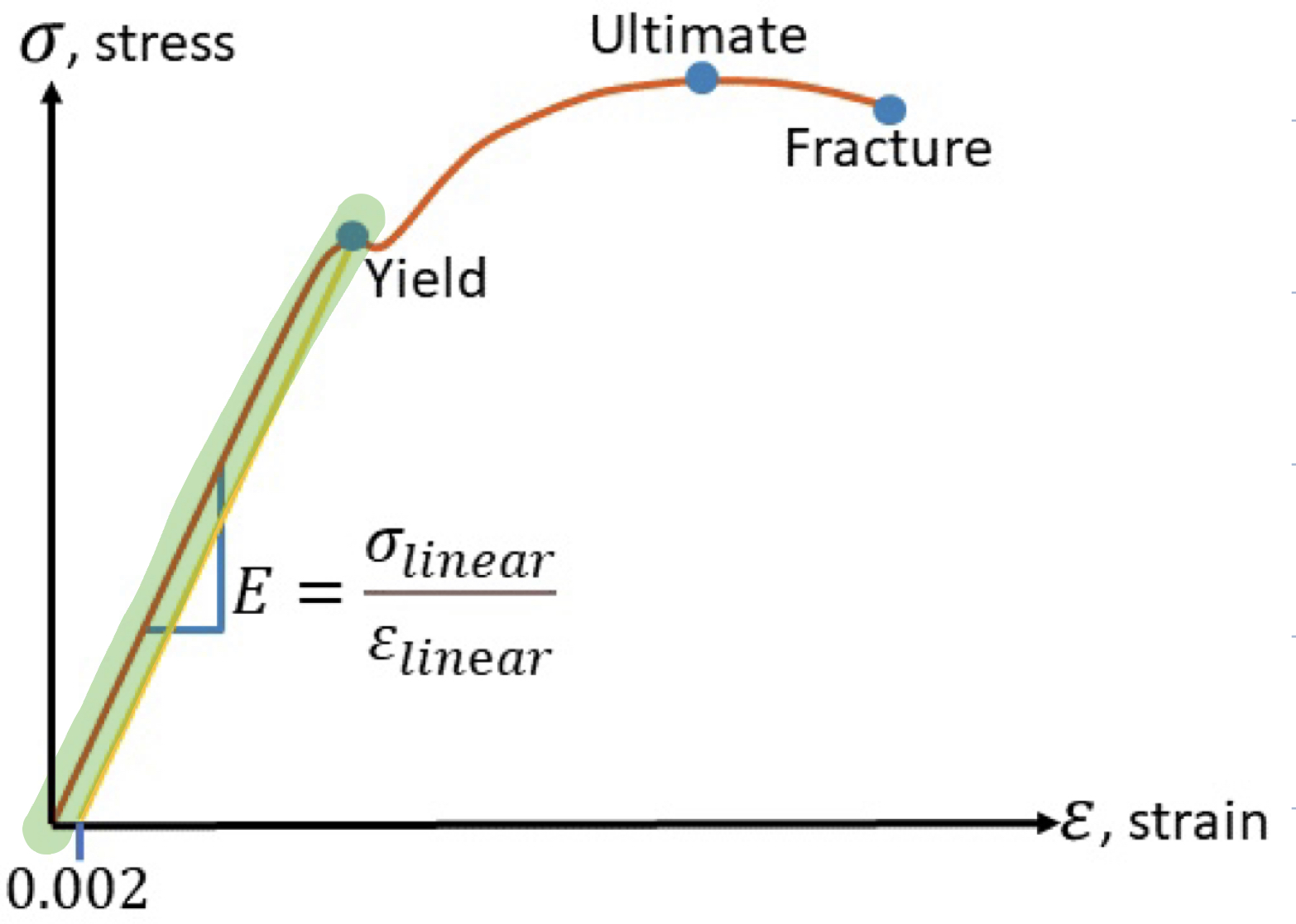
A stress-strain diagram is the relationship of normal stress as a function of normal strain. This diagram typically consists of a linear region, before the yield point, and a plastic region, after the yield point.

One way to collect these measurements is a uniaxial tension test in which a specimen is elongated at a very slow, constant rate (quasi-static). The applied load $ P $ and specimen length $ L $ are measured at frequent intervals.

Evaluation of average normal strain, or engineering strain (relative to undeformed length).

$$ \varepsilon = \frac{\delta}{L_0} = \frac{L-L_0}{L_0}\ $$

Evaluation of average normal stress, or engineering stress (relative to undeformed cross section).

$$ \sigma = \frac{P}{A_0}\ $$

Warning: Two stress-strain diagrams for a particular material will be similar, but not identical. #str-stn

Things that effect the material properties include imperfections, different composition, rate or loading, or temperature.

Extra!

There are many types of complex material behaviors. A few of them are listed below.

Anisotropy:

Isotropic: material properties are independent of the direction
Anisotropic: material properties depend on the direction (ie; composites, wood, and tissues)

Nonlinearity:

Some types of nonlinear material behaviors include viscoelasticity and creep, which introduce time dependency to the material response to loads. An example of this is silly putty, which is a viscoelastic, Non-Newtonian fluid. Silly putty behaves like a solid on quick impact, but flows slowly like a liquid over a long period of time.

Linear Elasticity

Elastic Modulus

Stress-strain diagram with linear region highlighted

Loading in this region results in elastic behavior, meaning the material returns to its original shape when unloaded. This region of the diagram is mostly a straight line, limited by the proportional limit. This region ends at $ \sigma_Y $ (yielding). For $ \sigma \le \sigma_{pl} $, the diagram is linear, and the behavior is elastic. For $ \sigma_{pl} < \sigma < \sigma_Y $, the diagram is nonlinear, but the behavior is still elastic. Hooke's law is used for small deformations in the elastic region. The Young's modulus (also known as the elastic modulus) is the slope $ E $.

Hooke's law.

$$ \sigma = E\varepsilon\ $$

Material	Young's modulus [$GPa$]
Mild Steel	210
Copper	120
Bone	18
Plastic	2
Rubber	0.02

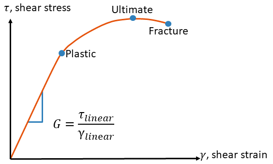
Shear Modulus

Shear stress strain diagram

Hooke's law.

$$ \tau_{xy} = G\gamma_{xy}\ $$

Shear modulus. #v_modulus

$$ G = \frac{E}{2(1+\nu)}\ $$

In the above equation, $\nu$ refers to Poisson's ratio. Only two of the three material constants (ie; $ G $, $ E $, $ \nu $) are independent in isotropic materials.

Poisson's Ratio

Poisson's ratio

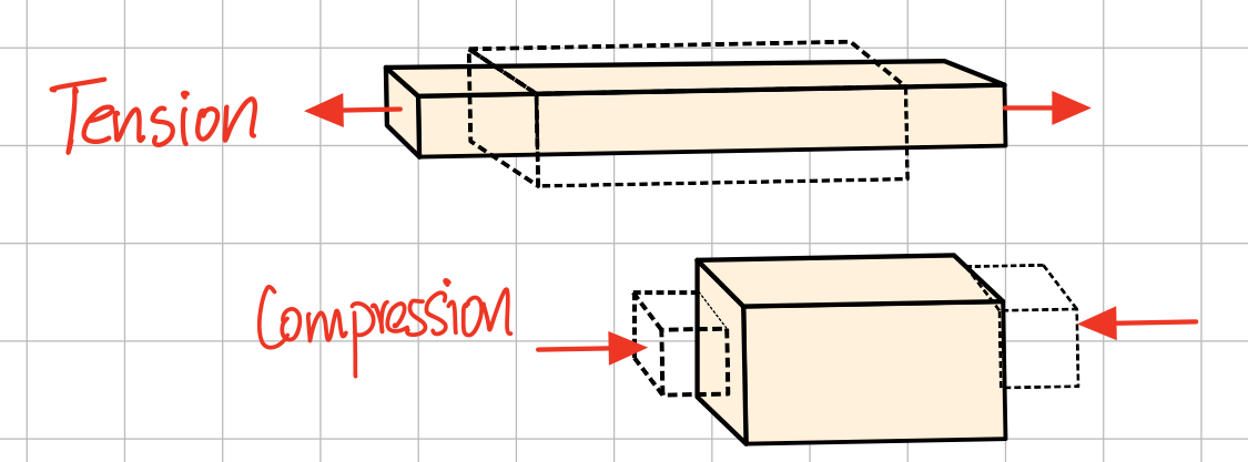
As illustrated in the figure above, when an object is being compressed it expands outward, and when stretched it will become thinner. Depending on the material, it may experience more or less lateral deformation for a given amount of axial deformation. The ratio that governs the amount of lateral strain per unit of axial strain is called Poisson's ratio.

Poisson's ratio $\nu$.

$$ \nu = -\frac{\text{lateral strain}}{\text{axial strain}} = -\frac{\varepsilon_y}{\varepsilon_x} $$

Typical range. #poisson_range

$$ 0 < \nu < 0.5\ $$

Consider a cylinder with volume $ V = A\cdot L $. We know that $ A = \frac{\pi}{4}d^2 $. Since the diameter is dependant on the change in length $dx$ due to Poisson's ratio, we get

$$ \frac{\partial A}{\partial x} = 2d\frac{\partial d}{\partial x}\frac{\pi}{4} = \frac{\partial d}{\partial x}\frac{\pi d}{2} $$

We use the chain rule to find the change in volume

$$ \begin{aligned} \frac{\partial V}{\partial x} &= \frac{\partial A}{\partial x}L + \frac{\partial L}{\partial x} A \\ &= \frac{\partial d}{\partial x}\frac{\pi d}{2}L + L \frac{\pi d^2}{4} \end{aligned} $$

By definition,

$$ \nu = -\frac{\varepsilon_y}{\varepsilon_x} = -\frac{\frac{\partial d}{d}}{\frac{\partial L}{L}} = -\frac{\partial d}{d}\frac{L}{\partial L}= -\frac{\partial d}{d}\frac{L}{L\partial x} = -\frac{1}{d}\frac{\partial d}{\partial x} \implies \frac{\partial d}{\partial x} = -\nu d $$

Returning to our first equation,

$$ \begin{aligned} \frac{\partial V}{\partial x} &= \frac{\partial d}{\partial x}\frac{\pi d}{2}L + L \frac{\pi d^2}{4} \\ &= -\nu d \frac{\pi d}{2}L + L \frac{\pi d^2}{4} \\ &= -\nu \frac{\pi d^2}{2}L + L \frac{\pi d^2}{4} \\ &= \frac{\pi d^2L}{4}\left( 1- 2\nu \right) \\ &= V\left( 1- 2\nu \right) \\ \end{aligned} $$

Since $\partial V \geq 0$ and $\nu > 0$ in nicely behaved materials, $ 0 < \nu \leq 0.5$. In practice $\nu = 0.5$ only if the material is incompressible, thus in most materials $\nu < 0.5$.

Lateral strain.

$$ \varepsilon_{z} = \varepsilon_{y} = -\nu\varepsilon_{x}\ $$

Heads Up!

Though typically the Poisson ratio will be positive, there are some materials (known as auxetic materials) which have a negative Poisson ratio. This means that these materials expand in all directions when pulled.

For an interesting demonstration on auxetic materials, check out this video:

Plasticity

Stress-strain diagram with plastic region highlighted

Plastic material behaviors occur after the material has been exerted past its yield point. In this region, permanent deformation takes place. Different materials behave differently when plastically deformed, and one major classification for describing these differences is ductility.

Extra!

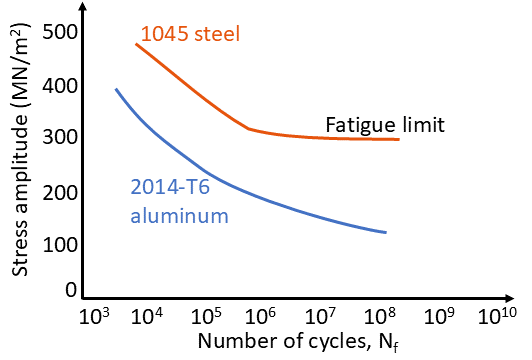
Fatigue builds on this content in Engineering Materials and Mechanical Design.

SN curve examples

If stress does not exceed the elastic limit, the specimen returns to its original configuration. However, this is not the case if the loading is repeated thousands or millions of times. In such cases, rupture will happen at stress lower than the fracture stress - this phenomenon is known as fatigue.

Ductility

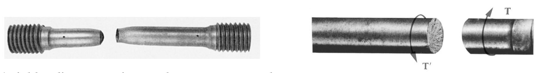
For ductile materials, tension failures occur along a cone shaped surface that forms an angle of approximately $ 45^\circ $ with the original surface of the specimen. Shear is primarily responsible for failure in ductile materials.

There are many ways to quantify ductility. A couple common ones are listed below.

Ways to quantify ductility. #mat-duct

$$ \begin{align} \text{% elongation} = 100 \times (L_f - L_o) / L_o \\ \text{% area reduction} = 100 \times (A_o - A_f) / A_o \end{align} $$

Extra!

Strain Energy builds on this content in Engineering Materials.

Deformation does work on the material: equal to internal strain energy (by energy conservation).

$$ \Delta U = \int F_{z}dz = \int \sigma_{z}(\Delta x \Delta y \Delta z)d\varepsilon_{z}\ $$

Energy density.

$$ u = \frac{\Delta U}{\Delta V} = \int \sigma_{z}d\varepsilon_{z}\ $$

Can be generalized to any deformation: areas under stress-strain curves

$$ u = \int \sigma d\varepsilon \quad \text{or} \quad u = \int \tau d\gamma\ $$

Yield Strength

Stresses above the plastic limit ($ \sigma > \sigma_Y $) cause the material to permanently deform. This limit is known as the yield strength .

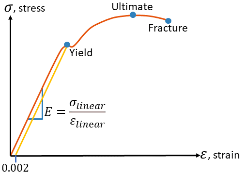
Perfect plastic or ideal plastic: well-defined $ \sigma_Y $, stress plateau up to failure. Some materials (e.g. mild steel) have two yield points (stress plateau at $ \sigma_{YL} $). Most ductile metals do not have a stress plateau; yield strength $ \sigma_{Y} $ is then defined by the 0.002 (0.2%) offset method.

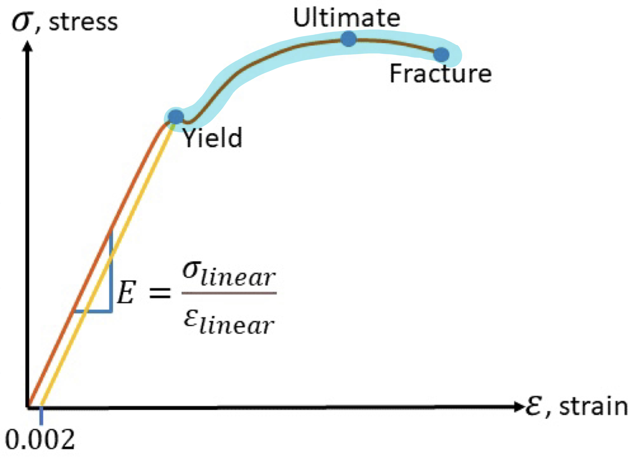
0.2% Offset Method

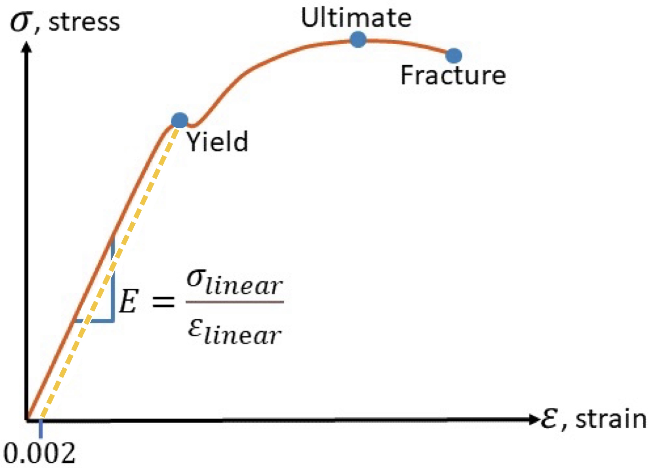
Stress-strain diagram with offset line highlighted

Note: The dotted yellow line above represents the 0.2% offset line for calculating yield stress.

On the stress-strain curve, the yield strength is the point at which the graph is no longer linear. However, most stress-strain curves will have a gradual shift from linearity to nonlinearity, making it difficult to identify an exact yield point. The 0.2% offset method allows for a consistent metric to determine where yielding in a material occurs.

Steps to perform the 0.2% offset method:

Determine the slope of the linear region of the stress-strain curve (the Young's modulus, E).
Start at 0.002 on the horizontal (strain) axis, and draw a line with slope E.
Find the point where the line from step 2 intersects the stress-strain curve. This is the 0.2% yield stress.

Strain Hardening

Strain hardening

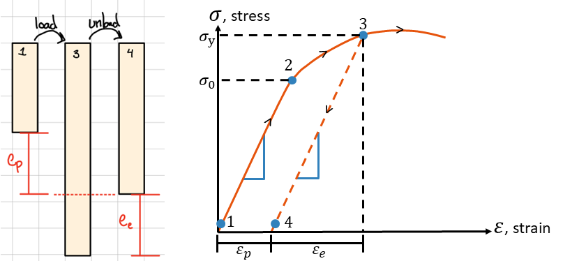
Atoms rearrange in plastic region of ductile materials when a stress higher than the yield strength is sustained. Plastic strain remains after unloading as permanent set, resulting in permanent deformation. Reloading is linear elastic up to the new, higher yield stress (at A') and a reduced ductility.

Ultimate Strength

The ultimate strength ($ \sigma_u $) is the maximum stress the material can withstand.

Necking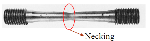

Necking

After ultimate stress ($ \sigma_u < \sigma $), the middle of the material elongates before failure. Necking only occurs in ductile materials.

Failure

Also called fracture or rupture stress ($ \sigma_f $) is the stress at the point of failure for the material. Brittle and Ductile materials fail differently.

Ductile materials generally fail in shear. There is a large region of plastic deformation before failure (fracture) at higher strain and necking.

Ductile failure

Axial – maximum shear stress at $45^o$ angle

Torsion – maximum shear stress at $0^o$ angle

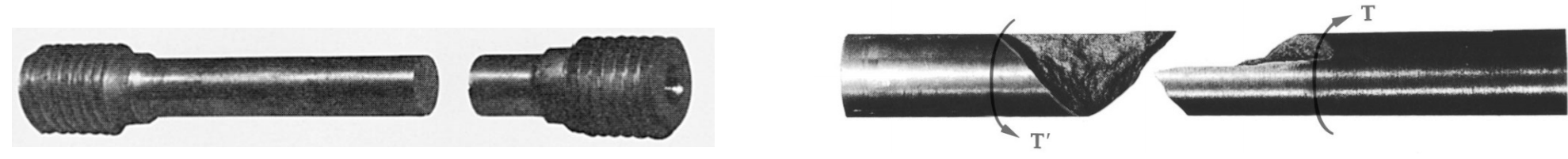
Brittle materials are weaker in tension than shear. There is a small plastic region between yield and failure (fracture) and no necking.

Brittle failure

Axial – maximum normal stress at $0^o$ angle

Torsion – maximum normal stress at $45^o$ angle

Note the difference between engineering and true stress/strain diagrams: ultimate stress is a consequence of necking, and the true maximum is the true fracture stress.

Example: Concrete is a brittle material.

Maximum compressive strength is substantially larger than the maximum tensile strength.
For this reason, concrete is almost always reinforced with steel bars or rods whenever it is designed to support tensile loads.

Brittle vs ductile failure

Whether a material is brittle or ductile can be shown from the stress strain curve. Ductile materials tend to have long plastic regions, such as graph (C) in the diagram above. Brittle materials lack a substantial plastic region, such as in graph (A) above.