Fatigue Introduction
Fatigue is a common type of failure for ductile materials under cyclical loads, caused by the formation of small cracks and the propagation of those cracks under a large number of loading cycles. It is important to account for fatigue in designs as the stresses needed for fatigue failure are often far lower than those that would be needed to cause plastic failure. This document covers fatigue theory and the methods to analyze the risk of fatigue failure in a mechanism.
Fatigue Theory
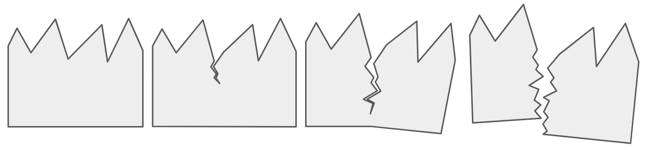
Fatigue occurs when cyclical loading allows a series of dislocations to line up and form a slip band. Sometimes when the slip plane intersects with a free surface on an object, it can cause a small crack to form. As the cyclical loading continues, the crack can slowly grow and cause catastrophic failure.
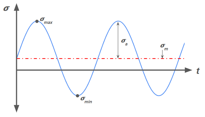
To characterize a cyclical load, there are two key parameters: Stress amplitude \( \sigma_a \) and mean stress \( \sigma_m \).
Stress amplitude describes the magnitude of change in stress within a cycle. It is defined with the equation
Mean stress describes how much stress is experienced on average within a cycle. It is defined by
Here, \( \sigma_{max} \) and \( \sigma_{min} \) are the maximum and minimum stress values reached in the cycle, respectively.
As intuition would suggest, the higher the stress amplitude on a specimen, the fewer cycles it can withstand before failing. This relationship has been examined in carefully designed experiments and expressed in S-N curves, plots of standard fatigue strength (S) vs number of cycles (N).

For some materials, including many steels, the S-N curve has asymptotic behavior as the number of cycles becomes very large, like in the figure above. This feature suggests that there is a certain stress threshold where the material could theoretically withstand an infinite number of cycles. This threshold is called the endurance limit.
There are two different expressions for the criteria to avoid failure depending on the mean stress value. The simplest case is when \( \sigma_m=0 \), where the criterion is
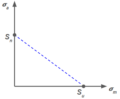
If the load has a nonzero \( \sigma_m \), the criterion instead follows the "Goodman Equation":
where \( S_u \) is the ultimate tensile strength and \( S_n \) is the endurance limit. This equation can be visualized with a "Goodman line," which connects \( S_n \) on the \( \sigma_a \) axis with \( S_u \) on the \( \sigma_m \) axis.
This line It forms a part of the broader "Infinite Life Diagram," which accounts for both fatigue and yield conditions. To construct the diagram, a flat line is extended from the top of the Goodman line as a conservative estimate of the fatigue failure condition under compression. Additionally, "yield lines" are plotted by connecting the value of the yield strength \( \sigma_y \) on each axis:

For a part to avoid failure, the stress state \( (\sigma_m, \sigma_a) \) must lie below both the yield line and the Goodman (fatigue) line:

To make the criteria above useful, we need to know how to calculate the endurance limit. It is calculated based on the material and external conditions, using the following equation:
One common point of confusion with this equation is differentiating \( S_n \) (true endurance limit) from \( S_n' \) (idealized endurance limit). \( S_n' \) is a known material property, whereas \( S_n \) must be calculated through accounting for conditions in the particular setup. A detailed explanation of each factor follows:
- \( S'_n \) - Idealized Endurance Limit:
- \( C_L \) - Load Factor:
- \( C_G \) - Gradient Factor:
- \( C_S \) - Surface Factor:
- \( C_T \) - Temperature Factor:
- \( C_R \) - Reliability Factor:
The idealized endurance limit is the maximum possible value for endurance limit of a material. It is a material property, and the best way to find it is through real data on a S-N curve. It can also be roughly approximated with a known ultimate strength or hardness. For ductile steel specifically, approximations follow:
| Expression | Unit |
|---|---|
| \( S_n'\approx 0.5 \cdot S_u \) | MPa or ksi |
| \( S_n'\approx 0.25 \cdot \)Bhn | ksi |
| \( S_n'\approx 1.73 \cdot \)Bhn | MPa |
The load factor accounts for the type of loading applied to the material. Fatigue life is greatly reduced under torsion compared to bending or axial loading, so \( C_L \) is smaller under torsion:
| Load Type | Bending | Axial | Torsion |
|---|---|---|---|
| \( C_L \) | 1.0 | 1.0 | 0.58 |
For most types of loading, there is a gradient of stress between the center and outer edge of the material. This gradient benefits the life of a material, but it does not benefit all setups equally. The gradient factor accounts for the fact that the gradient benefit is reduced for axial loading and for thicker beams:
| Load Type | Bending | Axial | Torsion |
|---|---|---|---|
| \( C_L (d < 10 mm) \) | 1.0 | 0.7-0.9 | 1.0 |
| \( C_L (10 mm < d < 50mm) \) | 0.9 | 0.7-0.9 | 0.9 |
Note that these are merely the typical suggested values as the gradient effect is complex. Also note that in the table, \( d \) represents effective diameter, a characteristic length that depends on the shape of the beam.
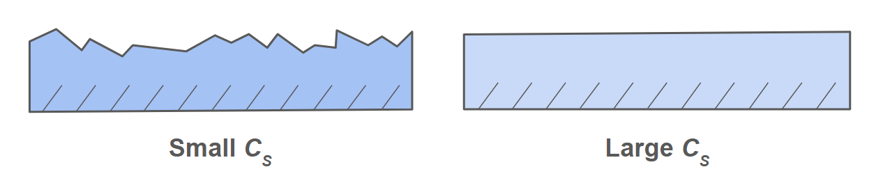
The surface factor accounts for a specimen's surface smoothness. A rough surface contains many defect sites that are vulnerable to crack propagation. Also, the stronger a material is, the greater the impact these defects make. Specific \( C_S \) values can be found in a textbook.
The temperature factor accounts for crack sensitivity at high temperatures. For steel at temperatures below 840F, \( C_T \) is assumed to be 1. Above 840F, we use the formula
Note that this formula is applicable to ductile steels only.
Due to the random nature of crack propagation, calculated endurance limits are merely approximations that do not predict the exact point at which every specimen will fail. The required reliability of a design needs to be evaluated, and the endurance limit should be lowered accordingly by applying the reliability factor, akin to a factor of safety:
| Desired Reliability | \( C_R \) |
|---|---|
| 50% | 1.000 |
| 90% | 0.897 |
| 95% | 0.868 |
| 99% | 0.814 |
| 99.9% | 0.753 |
If each correction factor has a value of 1.0, the endurance limit \( S_n \) is equal to the standard fatigue strength \( S_n' \). Thus, the correction factors can be seen as an account of adverse effects within the setup increasing the likelihood of defect propagation and reducing the real-world endurance limit.
Fatigue with Stress Concentrations:Just like with static stresses, the risk of fatigue failure is worsened in the presence of stress concentrations. These effects are quantified with the fatigue stress concentration factor \( K_f \), related to the ordinary stress concentration factor \( K_t \) through the following equation:
Here, \( q \) is called the notch sensitivity factor. It ranges between 0 and 1, and it increases with the size of the notch present and the material hardness.
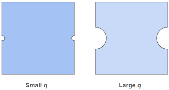
On careful observation, you may notice that \( K_f \leq K_t \). Though the underlying reasons are outside the scope of these pages, stress concentrations do not affect fatigue stresses as much as static stress. Like \( K_t \), however, \( K_f \) serves as a multiplier for the effective stress, adjusting \( \sigma_a \) and \( \sigma_m \) as follows:
In the best case, \( q=0 \), and thus \( K_f=1 \), and the stresses are unaffected. With extreme notch sensitivity, \( q \approx 1 \), so \( K_f \approx K_t \), signaling large effective stresses. Using the modified \( \sigma_a \) and \( \sigma_m \), failure criteria are applied in the usual way.