Solid Mechanics Review Introduction
To master topics related to machine failure, it is important to have a solid baseline intuition with concepts from introductory engineering mechanics, especially static loading and the resulting stresses produced in solid bodies. This document covers these topics as a preliminary review before the core material of the course.
Loads on Machines
Free-Body Diagrams
The first step in solving any loading problem is drawing a Free-Body Diagram (FBD). To consistently create reliable diagrams and avoid small errors, one should follow these steps:
- Show the general shape of the body under consideration
- Display all forces and moments acting on it
- Include relevant dimensions and angles
When one body exerts a force on another, we use an index convention where the first subscript is the body the force acts on, and the second subscript is the body exerting the force:
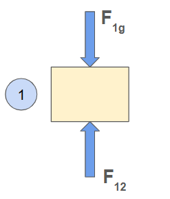
Two boxes are stacked on the ground. Draw a free body diagram for each box.
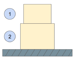
For Box 1, there is a downward gravitational force and an upward contact force from Box 2. The FBD should look like this:
For Box 2, there is a downward gravitational force, a downward contact force from Box 1, and an upward contact force from the ground. The FBD should look like this:
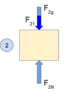
Note the index notation in each diagram. The force on box 2 from box one is labeled as \( F_{21} \) and vice versa.
Equilibrium Equations:>
When analyzing static loading on machines, we assume they are in equilibrium. With these conditions, the following equations apply:
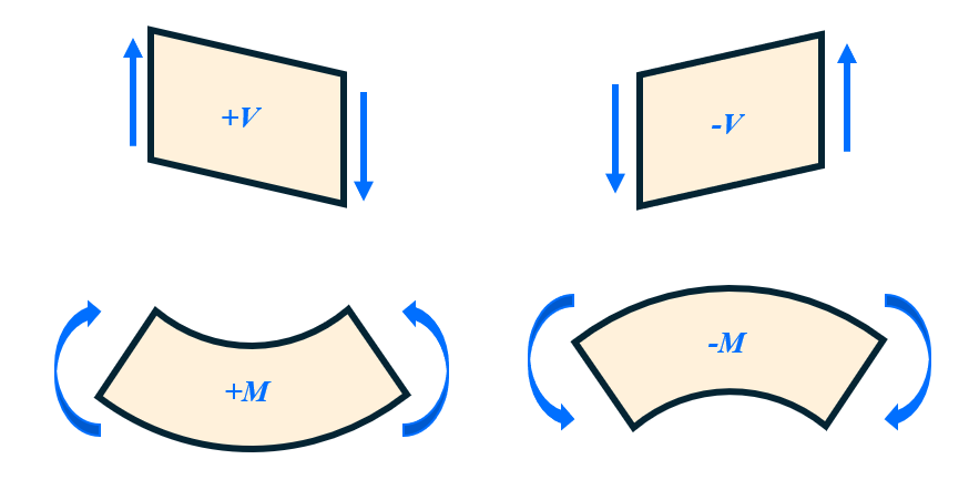
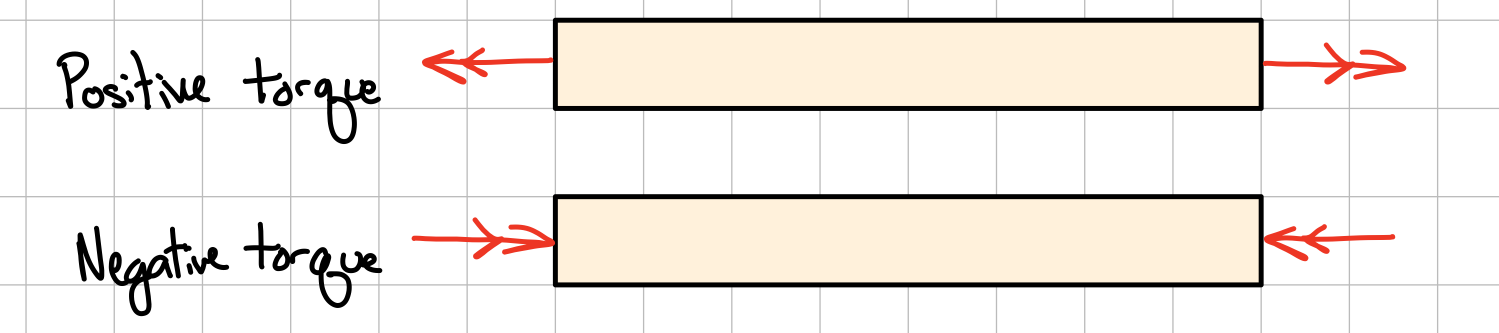
To study the way materials respond to loads, it is crucial to identify the resulting internal forces within the object, including normal force, shear force, and bending moment. To draw internal loads consistently, one should follow this sign convention:
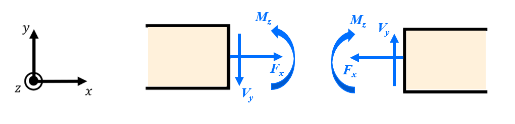
According to the sign convention, a segment experiencing positive shear force will have a downward slant, and one experiencing positive bending moment will have an upward curve:
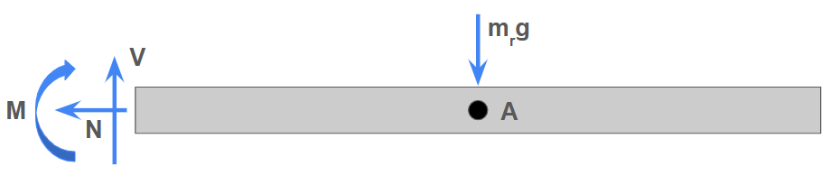
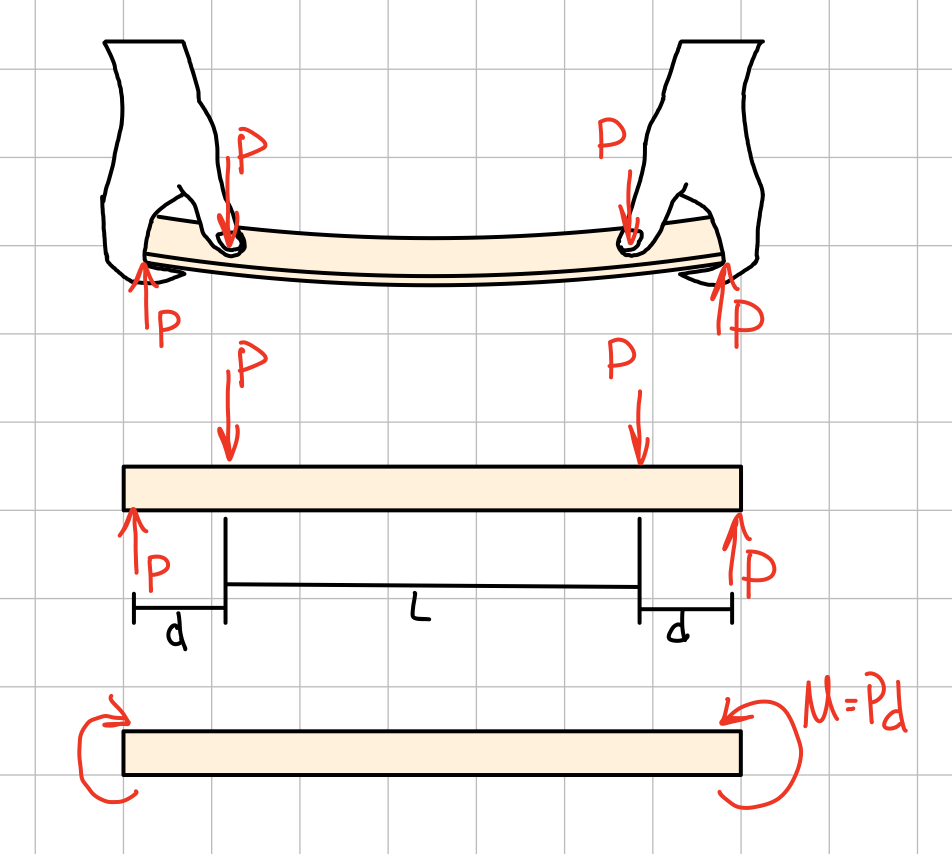
A rock of mass \( m_r \) sits on the center of a massless cantilever beam of length L. Find and analyze the normal load, shear load, and bending moment at the left end of the beam.

We start by creating a free body diagram of the beam, using the following information from the setup:
- Forces include the weight of the rock and the reaction forces from supports.
- Fixed support on left side - vertical force, horizontal force, and bending moment
- No support on right side - no reaction forces
Additionally, to maintain a consistent approach, we will assume each of the reaction loads are positive and draw them according to the sign convention. The resulting FBD looks like this:
Additionally, to maintain a consistent approach, we will assume each of the reaction loads are positive and draw them according to the sign convention. The resulting FBD looks like this:
Next, we can use this FBD and the three key equilibrium equations to find each load on the left end of the beam.
Horizontal:
Apply the equilibrium equation in the horizontal direction.
Vertical
Apply the equilibrium equation in the vertical direction.
Moment
To apply the moment equilibrium equation, we need to calculate the moment about a specific point. One convenient strategy is to choose the point at the center of the beam (as in point A marked in the FBD). Then, the weight of the rock has no effect on the moment, and the resulting equation follows:
Note that the shear (vertical) force is positive as assumed, while the bending moment is negative. Looking back at the sign conventions, this means the beam should experience a downward slant and a downward bend on the left end:
This aligns with intuition as we would imagine the beam to deflect downward if pushed down from the center.
Work and Power
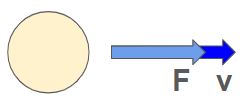
As you may remember from introductory physics courses, power is the rate of change of energy transfer over time. It can be described by the equation
where \( F \) is the force applied at a point, \( V \) is the velocity of that point, \( \theta \) is the angle between \( F \) and \( V \), and \( \dot{W} \) is the power transferred.
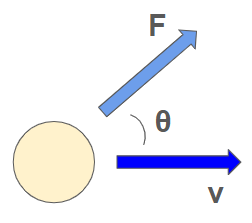
Assuming that the force and velocity are parallel, the equation simplifies to
Making sure to use consistent units, conversion factors can be built into the formula, as shown in this table:
| Unit System | Metric | Imperial |
|---|---|---|
| Formula | \( \dot W = \frac{F V}{1000} \) | \( \dot W = \frac{F V}{33,000} \) |
| Force Unit | \( N \) | \( lbf \) |
| Velocity Unit | \( m/s \) | \( ft/min \) |
| Power Unit | \( kW \) | \( hp \) |
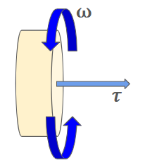
Gear Torque/Speed Ratios
In the analysis of rotating objects, power can be calculated with the equation
where \( \tau \) is the torque applied to the object and \( \omega \) is its rotational speed.
In a system of gears with negligible frictional losses,
Rearranging this expression, we get
Note that these are just magnitudes. The signs of the angular velocities and torques may change depending on the setup of the system.
Types of Stress
Stress Elements
To represent the state of stress at a chosen point on an object, we draw infinitesimal stress elements. Two-dimensional stress elements for objects with both normal and shear stresses will look something like this:
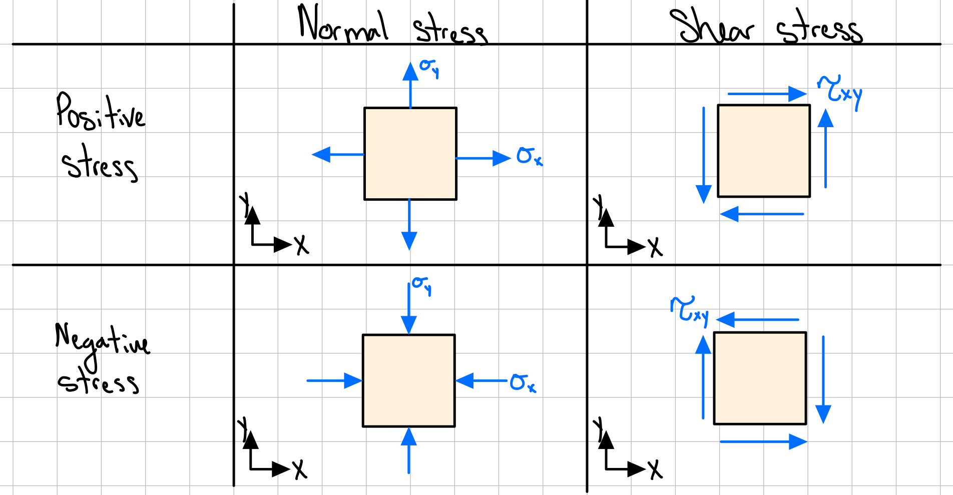
If the object has a three-dimensional stress state, the stress element will take the form of a cube instead, like this:
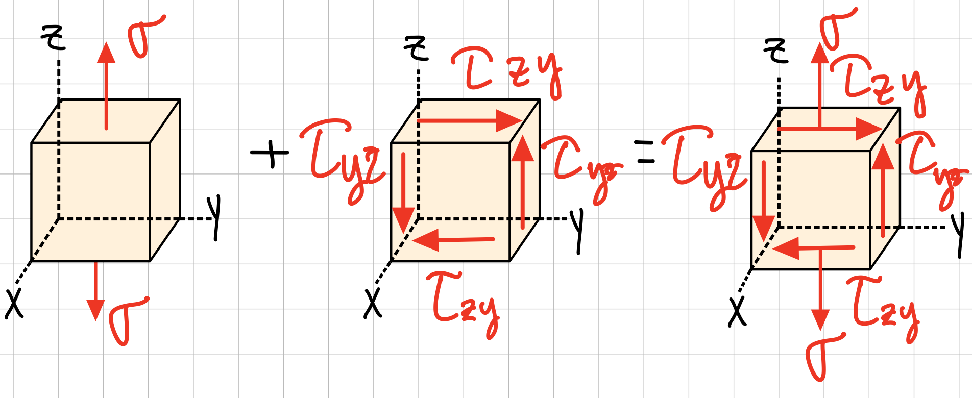
Notice that positive normal stress is indicated with arrows pointing outward from the faces, and positive shear stress is indicated with arrows converging on the top-right and bottom-left edges.
Also note that each shear stress is represented by four arrows lying in the same plane, which is required to cancel out the moments in the element, as expected for an object in equilibrium.
Axial Stress
Axial stress is a type of normal stress results from direct normal loading - tension and compression.
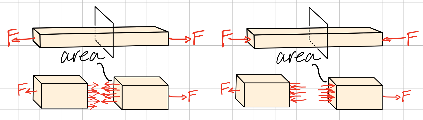
The axial stress is distributed evenly at every point across the face, given by:
where \( F \) is the internal normal force and \( A \) is the area of a cross section normal to the force.
Bending Stress
A bending moment creates an uneven distribution of normal stress across the face of a beam.
Bending stress at a point is a function of distance from the neutral axis, given by the equation
where \( M \) is the bending moment, \( y \) is the distance above the neutral axis, and \( I \) is the second moment of area of the cross section.
Notice that with a positive bending moment, at the top of the beam (positive y) there will be a negative stress. This aligns with our sign convention where a positive bending moment represents an upward bend, so the top of the beam is compressed while the bottom is stretched.
Torsional Stress
A torsion (twisting) force on a beam will also cause an uneven stress distribution. However, it will create a shear stress, not a normal stress.
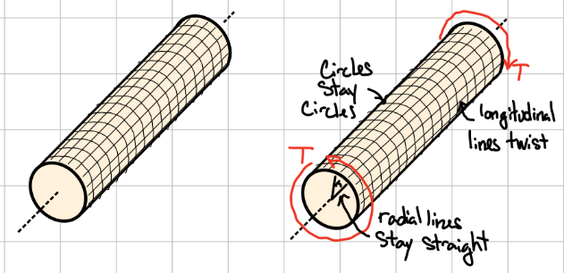
Generally, stress is greater for areas of the object farther from the axis of rotation. The shear stress at a point on a cylinder is given by the formula
where \( T \) is the applied torque, \( r \) is the distance from the central axis, and \( J \) is the polar moment of inertia of the cross section.
Transverse Shear
Transverse shear stress is caused by forces acting perpendicular to the axis of a beam.
This type of stress is also not uniform across the cross section, but unlike bending and torsional stress, it is highest at the center of the beam and lowest at the edges. Transverse shear stress at a point is given by the formula
Where \( Q \) is the first moment of area for the part of the cross section between the point and the edge of the beam, \( I \) is the moment of inertia of the entire cross section, \( V \) is the total shear force, and \( t \) is the thickness.
Stress Transformations
Mohr's circle in 2D and 3D (review or reuse materials from TAM)
\bigskip
Principle Stress
If we rotate our coordinate system around a stress element, it changes which stresses as normal stresses vs shear stress. For any state of stress, it is possible to find an angle where the normal stress is maximized and there is no shear stress. These maximized normal stresses are known as principle stresses, and the angle of the coordinate system with respect to the original system is the principle angle.
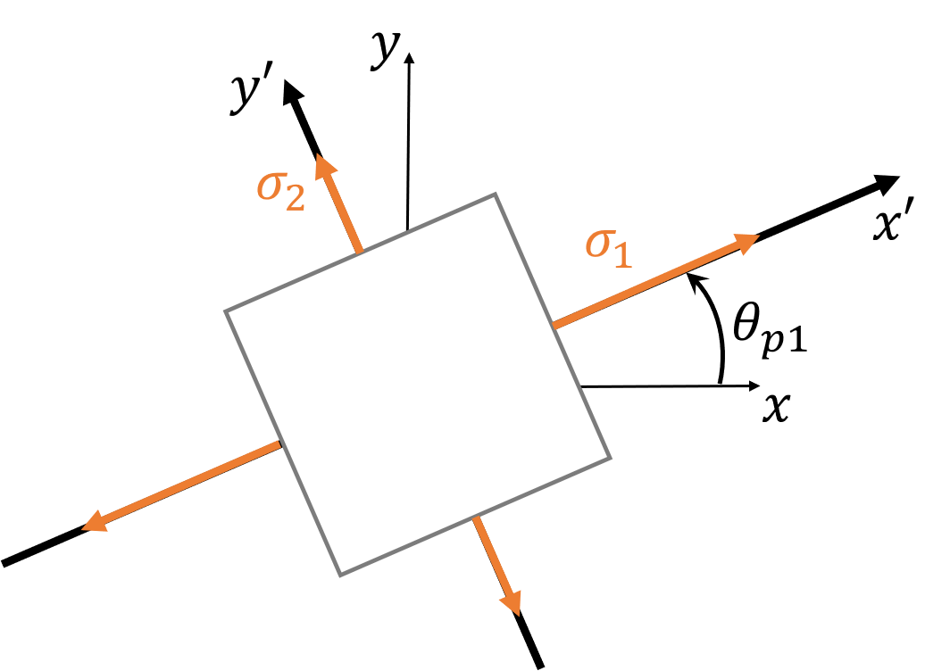
With known normal and shear stresses in one coordinate system, the principle stresses and principle angle can be directly calculated with these formulas:
Maximum Shear Stress
We can also find a coordinate system with maximum shear stress. However, at the point of maximum shear stress, the normal stresses do not disappear. Instead, this is the point of average normal stress, where the normal stress on one axis is equal to that of the perpendicular axis.
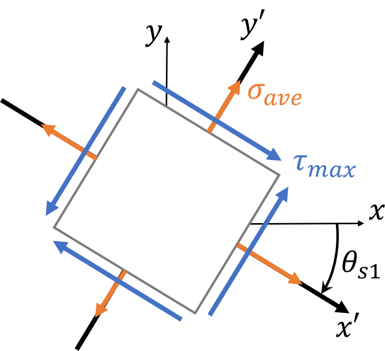
To calculate the maximum shear stress and angle, use these formulas:
Mohr's Circle
Mohr's circle is a graphical representation of stress transformations. The equations for stress transformations actually describe a circle if we consider the normal stress \( \sigma \) to be the x-coordinate and the shear stress \( \tau \) to be the y-coordinate.
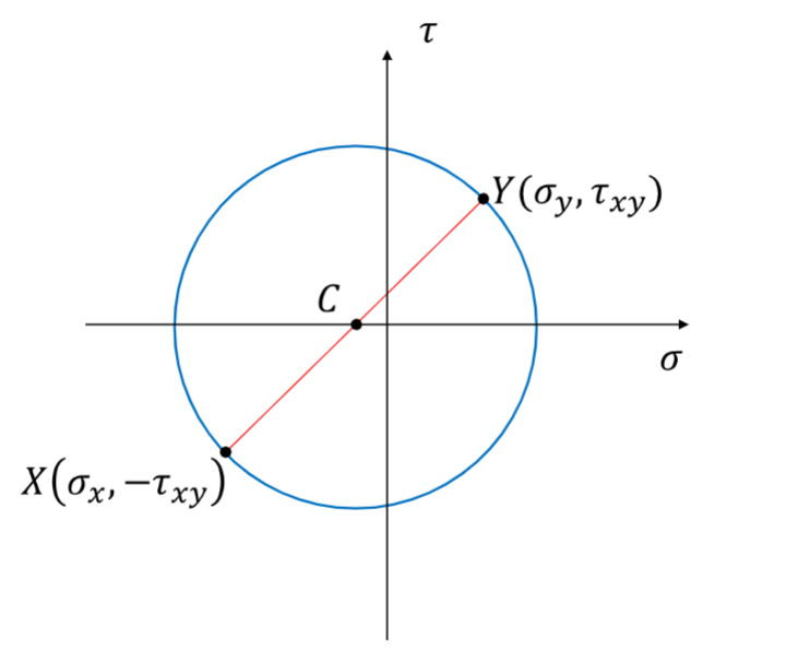
Here, we choose two points to form opposite ends of a circle: point \( X \) at \( (\sigma_x, -\tau_{x,y}) \) and point Y at \( (\sigma_y, \tau_{x,y}) \). With this constructed circle, we can easily find the principle stresses and maximum shear stress using the x-value of the center point \( C \) and the length of the radius \( R \). More precisely, the following relationships are true:
Mohr's Circle in 3D
In reality, every stress state has stresses in three dimensions and therefore has three principle stresses. When we bring in 3D stress transformations, we get some new insights, even if \( \sigma_3=0 \).
To construct Mohr's Circle in 3D, we need to draw three circles using the known principle stresses in each dimension:
- Connect \( \sigma_1 \) and \( \sigma_2 \)
- Connect \( \sigma_2 \) and \( \sigma_3 \)
- Connect \( \sigma_1 \) and \( \sigma_3 \)
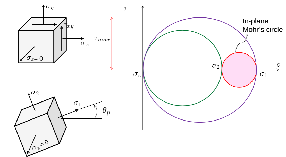
Just as the radius of original circle (connecting \( \sigma_1 \) and \( \sigma_2 \)) represents the maximum in-plane shear stress, the radius of the largest circle represents the maximum absolute shear stress.
Note that \( \sigma_3 \) is not always \( \sigma_z \). By convention, the principle stress with the highest value is labeled \( \sigma_1 \), and the one with the lowest value is labeled \( \sigma_3 \).