Introduction
In previous chapters, fluid mechanics problems were primarily analyzed by applying conservation laws to systems or control volumes. While these governing equations provide a complete mathematical description of fluid flow, many engineering problems involve several interacting variables such as velocity, pressure, density, viscosity, gravity, and geometry that combine in complex or nonlinear ways. As was seen, these effects make the formulation of analytic solutions extremely difficult. Moreover, as the number of variables increases, it becomes more difficult to determine which physical effects actually dominate the flow behavior.
Dimensional analysis provides a systematic method for simplifying these problems by combining variables into dimensionless groups. Rather than studying each dimensional quantity independently, the flow may instead be described using parameters that compare competing physical effects, such as inertial, viscous, gravitational, or compressibility effects.
A major tool used in this process is the Buckingham Pi Theorem, which states that a problem involving several dimensional variables may be rewritten in terms of a smaller set of independent dimensionless groups called \( \pi \) terms.These groups help reduce problem complexity, organize experimental data, and develop generalized relationships between variables.
Dimensionless parameters also form the basis of similitude and scale modeling. In many engineering applications, full-scale systems are too expensive or impractical to test directly, so smaller laboratory models are used instead. If the correct similarity conditions are satisfied, the behavior of the model can be used to predict the behavior of the full-scale prototype.
This chapter develops the Buckingham Pi Theorem, introduces common dimensionless groups used in fluid mechanics, discusses experimental correlations and scale models, and shows how important dimensionless parameters may also emerge directly from the governing equations through non-dimensionalization.
Motivation
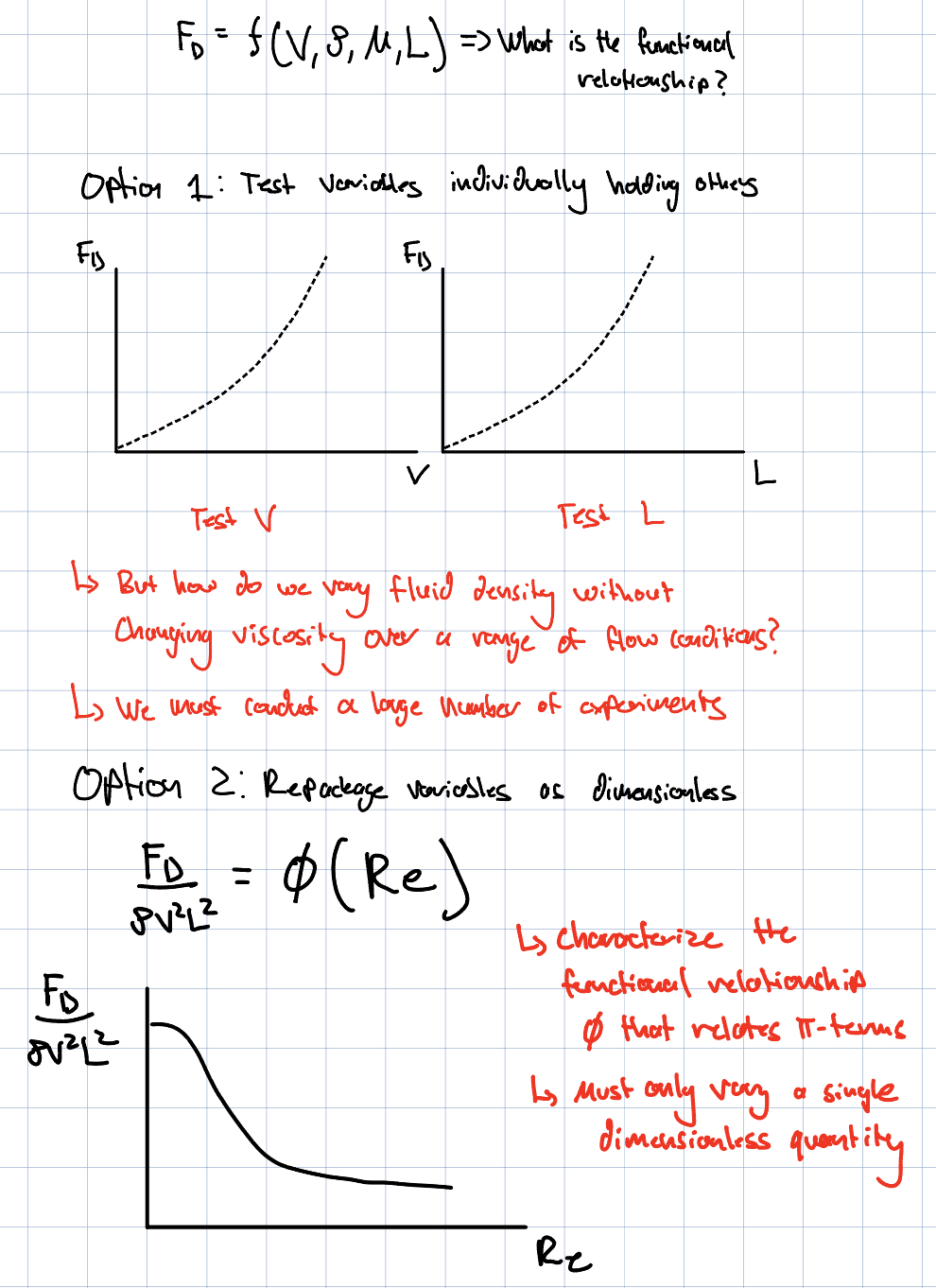
In many fluid mechanics problems, the primary goal is to determine how one quantity depends on several others. For example, the drag force acting on an object moving through a fluid may depend on the fluid velocity, density, viscosity, and the size of the object. Symbolically, this relationship might be written as
While conservation laws and governing equations may fully describe the flow, solving those equations directly is often difficult or impractical for real engineering systems. In addition, experimentally studying every variable independently would require a large number of tests. Dimensional analysis helps simplify this process by combining variables into dimensionless groups. Rather than searching for a relationship between many dimensional quantities, the problem may instead be rewritten in terms of a smaller set of dimensionless parameters. This reduces problem complexity while still preserving the important physical behavior of the flow.
Expressing results in dimensionless form is also useful because experimental data obtained from one system can often be applied to other similar systems. This idea forms the basis for experimental correlations, scale models, and similitude in fluid mechanics.
Buckingham Pi Theorem
The Buckingham Pi Theorem is a method for rewriting a dimensional physical relationship in terms of dimensionless groups. These dimensionless groups are called \( \pi \) terms. The main idea is that a problem with many dimensional variables can usually be described using fewer dimensionless parameters. It is then possible to conduct experiments that specify only the value of these dimensionless combination of variables as opposed to the individual value of each dimensional variable to identify the functional relationship between the dimensionless quantities. The Buckingham Pi Theorem can be overviewed as follows:
Suppose a fluid mechanics problem depends on \( n \) dimensional variables:
are the dimensionless quantities known as Pi terms. They are a repackaging of the dimensional variables.
Note that the theorem does not give the exact function \( \phi \). In this way, dimensional analysis is not a method to solve or characterize the analytical relationship between variables. Instead, it identifies which dimensionless parameters the final relationship must depend on in a way that can greatly simplify empirical analysis.
Carrying Out the Buckingham Pi Theorem
The method of repeating variables is a common method for determining Pi terms and applying the Buckingham Pi Theorem. It can usually be broken down- List all variables expected to influence the problem.
- Write the dimensions of each variable using basic dimensions such as mass \( M \), length \( L \), time \( T \), and temperature \( \Theta \).
- Count the total number of variables, \( n \).
- Count the number of independent reference dimensions, \( r \).
- Determine the number of dimensionless groups using:
- Choose \( r \) repeating variables. These variables should collectively contain all fundamental dimensions and should not already form a dimensionless group by themselves.
- Combine each non-repeating variable with the repeating variables to form a \( \pi \) term. In general, a pi term takes the form:
- Solve for the exponents that make each \( \pi \) term dimensionless by setting the powers of each fundamental dimension equal to zero.
Example: Drag Force on a Body
Consider the drag force acting on a body moving through a fluid. Assume the drag force depends on velocity, fluid density, fluid viscosity, and a characteristic length (Chapter 9 will demonstrate a more complete relationship for drag):Finding Pi Terms by Inspection
In some problems, dimensionless groups can be identified without explicitly solving for unknown exponents. This approach is called finding \( \pi \) terms by inspection. After gaining experience with common fluid mechanics problems and dimensionless parameters, this method is often significantly faster than the full repeating variable procedure.
The basic idea is to look for combinations of variables that naturally form dimensionless ratios. Since the goal is to compare physical effects, many dimensionless groups arise from comparing quantities with similar units or similar physical meaning. For example:
Example: Drag Force by Inspection
Consider again the drag force acting on a body moving through a fluid:Key Dimensionless Groups
When working through the Buckingham Pi Theorem, one might notice that certian dimensionless quantities appear repeatedly. Indeed, many of these quantities aren't simple an convenient mathematical packaging, but rather carry with them physical significance. Many dimensionless groups appear repeatedly throughout fluid mechanics because they compare the relative importance of different physical effects. These parameters are useful for characterizing flow behavior, correlating experimental data, and establishing a connection between models of different scales or prototypes.
Additionally, as was already seen in Chapter 6, they are particulary useful in identifying when certain simplifying assumptions are valid such as neglecting viscous effects or assuming incompressibility, the entire foundation in most introductory fluid mechanics courses. To that end, the Reynolds number, the most important and common dimensionless quantity incompressible flow and the mach number, both of which have been mentioned in previous chapters, are reviewed again here.
Reynolds Number
The Reynolds number compares the relative magnitude of inertial effects or forces in a flow to viscous effects:- \( \rho \) is fluid density,
- \( V \) is a characteristic velocity,
- \( L \) is a characteristic length,
- \( \mu \) is dynamic viscosity,
- \( \nu \) is kinematic viscosity.
Mach Number
The Mach number compares flow velocity to the local speed of sound:- \( V \) is the flow velocity,
- \( c \) is the local speed of sound.
The Mach number measures the importance of compressibility effects within a flow For low Mach numbers, density changes are often negligible, while compressibility effects become increasingly important at higher Mach numbers. With this in mind, a typical incompressible flow analysis will usually not include the Mach number, however; as was stated in Chapter 1, it is vitally important to use the Mach number to consider whether an assumption about incompressibility is valid. Engineers who work on on high-speed flows or those involving transonic or supersonic flows such as those encountered in jet engines or turbines will see that many functional relationships between common flow variables become functions of the Mach number.
The following table provides an overview of some common dimensionless groups encountered in fluid mechanics. Whether or not a specific dimensional quantity is relevant for a fluids problem depends heavily on the nature of the problem, the working fluid, and the relevant forces at play. Additionally, as the last two entries demonstrate, dimensionless quantities also appear quite frequently in other related fields, such as thermodynamics and heat transfer. Many energy transfer mechanisms, particularity those involving convention depend on both heat transfer properties of materials but also flow properties and are therefore often referred to as thermo-fluidics problems. Many of the principles developed here for incompressible flow, can be naturally extended into heat transfer and other adjacent fields.
Notable dimensionless groups in fluid mechanics and heat transfer
| Name | Symbol | Definition | Primary Comparison |
|---|---|---|---|
| Reynolds Number | \( Re \) | \( \displaystyle Re=\frac{\rho V L}{\mu}=\frac{VL}{\nu} \) | Inertial / viscous effects |
| Mach Number | \( Ma \) | \( \displaystyle Ma=\frac{V}{c} \) | Flow speed / speed of sound |
| Froude Number | \( Fr \) | \( \displaystyle Fr=\frac{V}{\sqrt{gL}} \) | Inertial / gravitational effects |
| Euler Number | \( Eu \) | \( \displaystyle Eu=\frac{\Delta p}{\rho V^2} \) | Pressure / inertial effects |
| Weber Number | \( We \) | \( \displaystyle We=\frac{\rho V^2 L}{\sigma} \) | Inertial / surface tension effects |
| Strouhal Number | \( St \) | \( \displaystyle St=\frac{fL}{V} \) | Unsteady / convective effects |
| Prandtl Number | \( Pr \) | \( \displaystyle Pr=\frac{\nu}{\alpha} \) | Momentum diffusion / thermal diffusion |
| Nusselt Number | \( Nu \) | \( \displaystyle Nu=\frac{hL}{k} \) | Convective / conductive heat transfer |
Scale Models
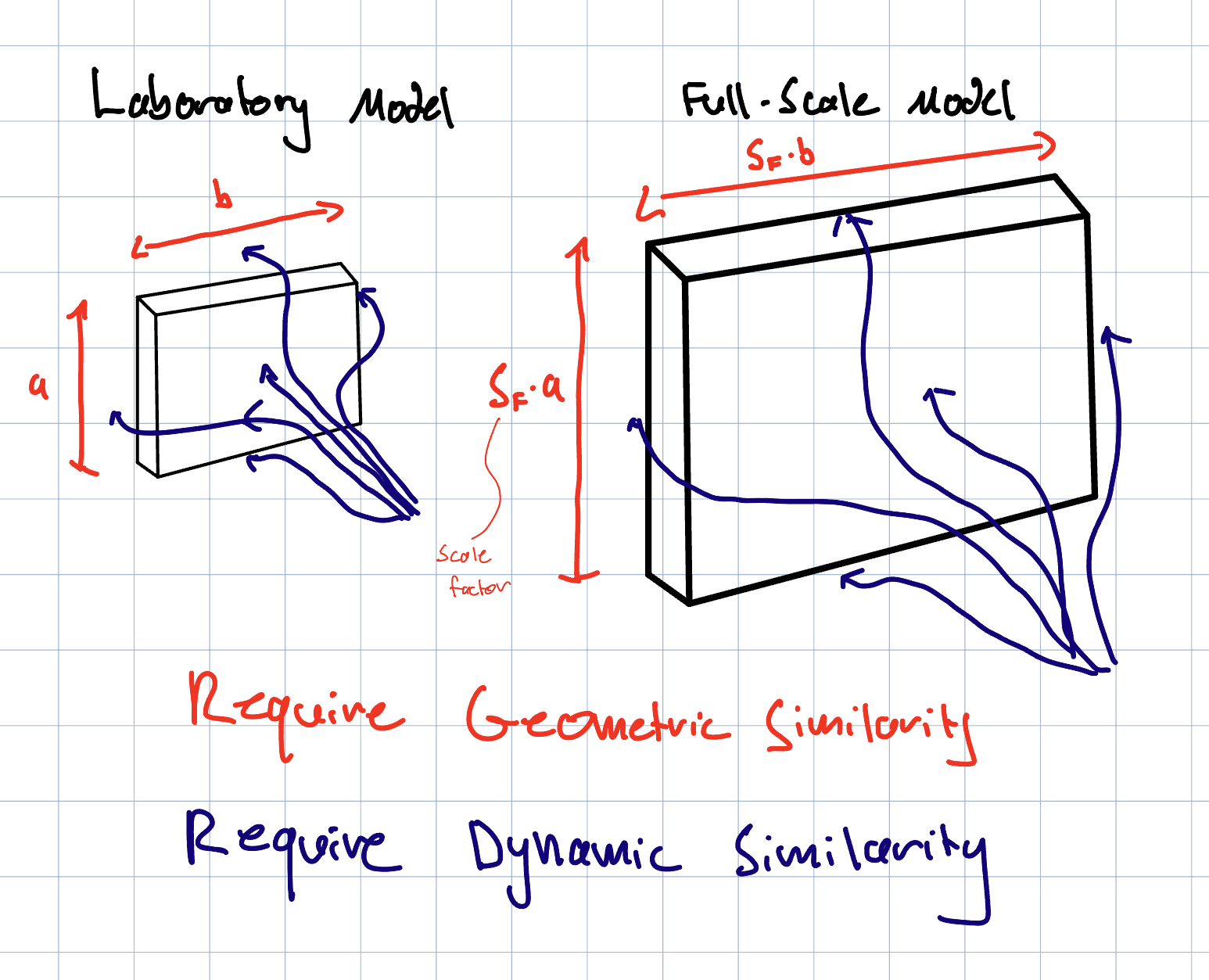
In many engineering applications, directly testing a full-scale system may be too expensive, impractical, or difficult to control. Instead, smaller laboratory models are often constructed and tested under controlled conditions, such as aircraft testing in wind tunnels.
The purpose of a scale model is not simply to create a smaller geometric copy of the real system, but rather to reproduce the important flow physics of the prototype. This is accomplished by matching the appropriate dimensionless groups between the model and the real system or in other words, equating pi terms. Given that a physical relationship is written in dimensionless form as:
Non-Dimensionalizing Equations
Another important application of dimensional analysis is rewriting governing equations and exact solutions in dimensionless form. This process is called non-dimensionalization.
The basic idea is to scale variables using characteristic reference quantities. For example, a velocity may be scaled by a characteristic speed \( V \), a length by a characteristic length \( L \), a time by a characteristic flow time \( L/V \), and a pressure by a characteristic pressure scale \( \rho V^2 \):
The starred quantities are dimensionless variables that have been normalized with respect to their reference quantities.
Once the dimensionless variables are defined, they are substituted into the original governing equations. The equations are then algebraically rearranged so that all remaining terms are dimensionless. During this process, dimensionless groups naturally emerge from the mathematics itself. For example, the incompressible Navier--Stokes equations may be written as:
is the now familiar Reynolds number. The reciprocal of the Reynolds number now appears directly as the coefficient multiplying the viscous term. Large Reynolds numbers therefore correspond to flows where inertial effects dominate, while small Reynolds numbers indicate flows where viscous effects are more important, just as was discussed earlier.
Dimensionless forms are also useful when rewriting exact solutions. For example, capillary rise (as was touched on in the introductory reference content) in a tube may be written as:
is the dimensionless height.
Expressing equations and solutions in dimensionless form generally doesn't chart new progress in solving an analytic equation. Nevertheless, it often simplifies the mathematics, highlights the dominant physics, and allows the results to apply to a broader class of similar flow problems.