Differential Fluid Flow

Introduction

In the previous chapter, conservation laws were applied using finite control volumes to analyze engineering fluid systems. While those integral formulations are extremely useful, many fluid mechanics problems require information about how flow properties vary continuously throughout the fluid domain.

This chapter develops the differential forms of the conservation equations by applying conservation principles to infinitesimally small fluid elements. These equations describe the local behavior of the flow field and form the foundation of theoretical fluid mechanics, computational fluid dynamics, and many advanced engineering analyses.

The chapter begins with the differential form of conservation of mass and introduces the stream function for incompressible two-dimensional flow. The differential equations of motion are then developed from conservation of linear momentum. Finally, the Navier--Stokes equations are introduced for viscous flows, followed by several classical analytical solutions for simple laminar flow configurations.

Motivation

Up until this chapter, various incarnations or consequences of Newton's Laws as they apply to fluid mechanics have been explored. However, for the most part, reframing the governing equations of mechanics have come with certain caveats and assumptions about a flow that permit the use of general formulae like the Bernoulli equation or special transformations of conservation principles like in RTT to aid in solving for specific flow properties at special locations. While a host of fluids problems can be effectively solved with these tools, it would be even more valuable to develop a stable method for fully solving any arbitrary fluids problem. That is, it is desirable to be able to apply a technique to solve for any fluid property (velocity, pressure, density, acceleration etc.) as a function of space and time while considering all forces, including gravity and viscous effects. Since it has been established that fluid mechanics is governed by the same overall laws as other areas of mechanics, it is not surprising that developing a general and complete solution strategy to fluid mechanics problems involves finding solutions to 2nd order, non-linear partial differential equations. In accordance with The Big Idea of Fluid Mechanics, these equations are nothing but Newton's 2nd Law and conservation of mass and energy expressed in differential form for infinitesimally small fluid domains.

Unfortunately, obtaining a closed-form analytical solution to these equations for most flows is, as of yet, not tractable. Nevertheless, the equations presented in this chapter represent some of the most general and foundational expressions of fluid flow behavior and understanding them is necessary to developing a robust intuition for fluid flow behavior and the origin of the equations that have been presented thus far. Also, while analytical solutions are often hard to find, it numerical methods can be used to obtain approximate, yet accurate solutions to many of these equations, allowing engineers to simulate complex flow fields to design systems.

Differential Conservation of Mass

The differential form of conservation of mass describes how mass is conserved locally within a fluid flow field. Instead of analyzing a finite control volume, the equations are written for an infinitesimally small fluid element. This approach allows the velocity, pressure, and density fields to be described continuously throughout the flow domain.

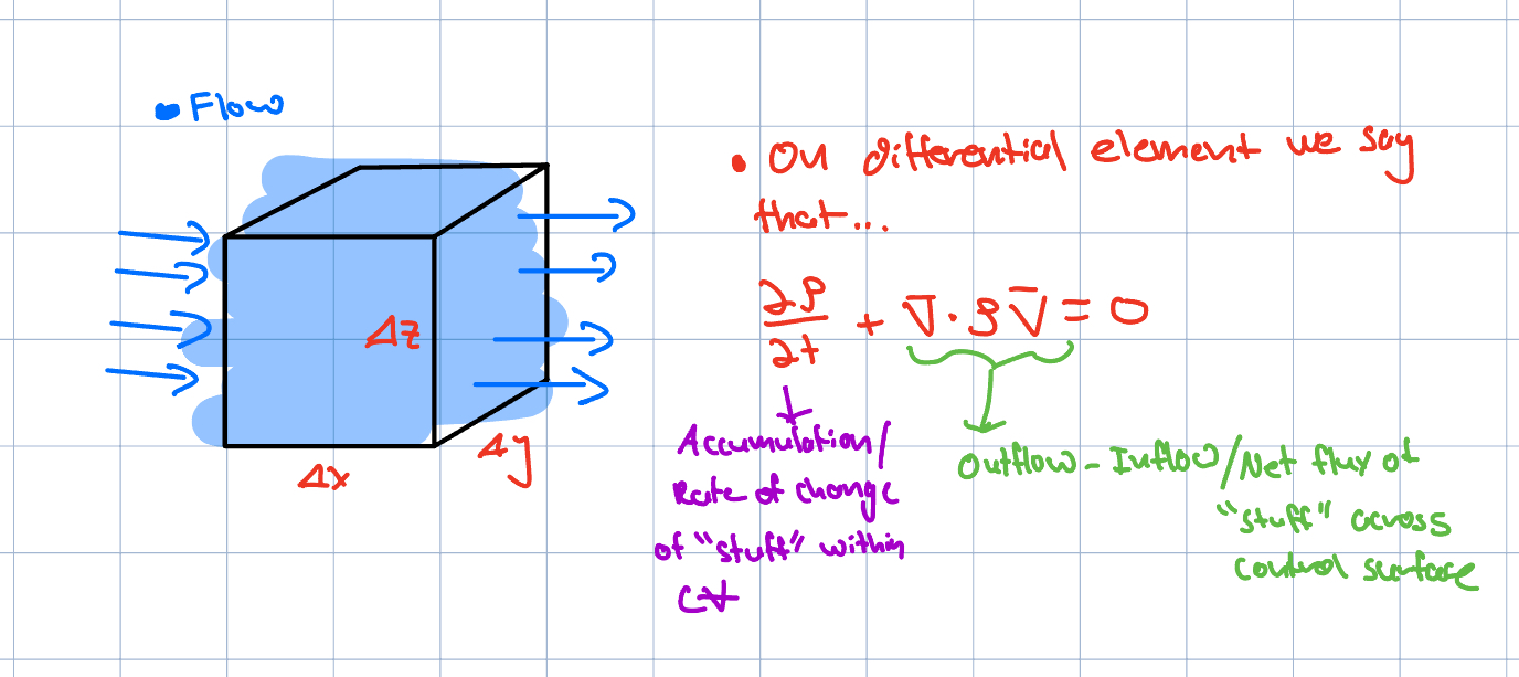
The general vector form of the continuity equation is

$$ \frac{\partial \rho}{\partial t} + \nabla \cdot (\rho \vec{V}) = 0 $$

This equation states that the rate of increase of mass inside a differential fluid element plus the net mass flow leaving the element must equal zero.

The first term represents local changes in density with time, while the second term, sometimes called the divergence term, represents the net mass transport caused by fluid motion.

Cartesian Coordinates

In Cartesian coordinates, the continuity equation becomes

$$ \frac{\partial \rho}{\partial t} + \frac{\partial (\rho u)}{\partial x} + \frac{\partial (\rho v)}{\partial y} + \frac{\partial (\rho w)}{\partial z} = 0 $$

Mass conservation on differential fluid element

For incompressible flow with constant density, the equation simplifies to

$$ \nabla \cdot \vec{V}=0 $$

or

$$ \frac{\partial u}{\partial x} + \frac{\partial v}{\partial y} + \frac{\partial w}{\partial z} = 0 $$

This expression is the same one that was overviewed briefly in Chapter 1. This expression states that an incompressible flow cannot experience a differential change in volume at any precise point or that it cannot accumulate in the differential control volume. Any fluid entering a differential element must be balanced by fluid leaving the element.

Cylindrical Polar Coordinates

Many engineering flows are more naturally described using cylindrical coordinates $(r,\theta,z)$, especially pipe flows and axisymmetric flows.

In cylindrical coordinates, the continuity equation becomes

$$ \frac{\partial \rho}{\partial t} + \frac{1}{r} \frac{\partial}{\partial r} (\rho r V_r) + \frac{1}{r} \frac{\partial}{\partial \theta} (\rho V_\theta) + \frac{\partial}{\partial z} (\rho V_z) = 0 $$

For incompressible flow,

$$ \frac{1}{r} \frac{\partial}{\partial r} (rV_r) + \frac{1}{r} \frac{\partial V_\theta}{\partial \theta} + \frac{\partial V_z}{\partial z} = 0 $$

Note that additional geometric factors arise because the coordinate directions themselves change with position in cylindrical systems. Note that when one switches the coordinate system that is used to analyze a fluid system, they must make an analogous change to the governing equations over that domain.

Stream Function

For two-dimensional incompressible flow, the continuity equation can be satisfied automatically through the introduction of the stream function, denoted by $\psi$.

In Cartesian coordinates,

$$ u=\frac{\partial \psi}{\partial y} $$

$$ v=-\frac{\partial \psi}{\partial x} $$

Substituting these expressions into the incompressible continuity equation identically satisfies conservation of mass.

The stream function is useful because lines of constant $\psi$ correspond to streamlines of the flow. Differences in stream function between two streamlines are related to the volumetric flow rate between them.

For axisymmetric incompressible flow in cylindrical coordinates,

$$ V_r = \frac{1}{r} \frac{\partial \psi}{\partial z} $$

$$ V_z = - \frac{1}{r} \frac{\partial \psi}{\partial r} $$

As a simple example, consider the stream function

$$ \psi=Ux $$

where $U$ is a constant velocity. The resulting velocity field is

$$ u=\frac{\partial \psi}{\partial y}=0 $$

$$ v=-\frac{\partial \psi}{\partial x}=-U $$

which represents uniform flow in the negative $y$-direction. Similarly, if

$$ \psi=Uy $$

then

$$ u=U \qquad \text{and} \qquad v=0 $$

which corresponds to uniform flow in the positive $x$-direction.

$$ \psi=Uy $$

where $U$ is a constant. Using the stream function definitions,

$$ u=\frac{\partial \psi}{\partial y}=U $$

$$ v=-\frac{\partial \psi}{\partial x}=0 $$

This corresponds to uniform flow in the positive $x$-direction. Substituting these velocity components into the incompressible continuity equation,

$$ \frac{\partial u}{\partial x} + \frac{\partial v}{\partial y} = 0 $$

gives

$$ \frac{\partial U}{\partial x} + \frac{\partial (0)}{\partial y} = 0 $$

or

$$ 0+0=0 $$

showing that the continuity equation is satisfied automatically.

Differential Equations of Motion

The differential equations of motion describe how fluid motion changes in response to forces acting on a differential fluid element. Again, these equations are obtained by applying Newton's Second Law locally or at given locations within the flow field.

The equations of motion form the foundation of fluid dynamics because they relate velocity, pressure, viscosity, and body forces throughout the fluid domain.

The general vector form is

$$ \rho \frac{D\vec{V}}{Dt} = -\nabla p + \nabla \cdot \boldsymbol{\tau} + \rho \vec{g} $$

Using the material derivative reviewed in Chapter 4 in its vector form,

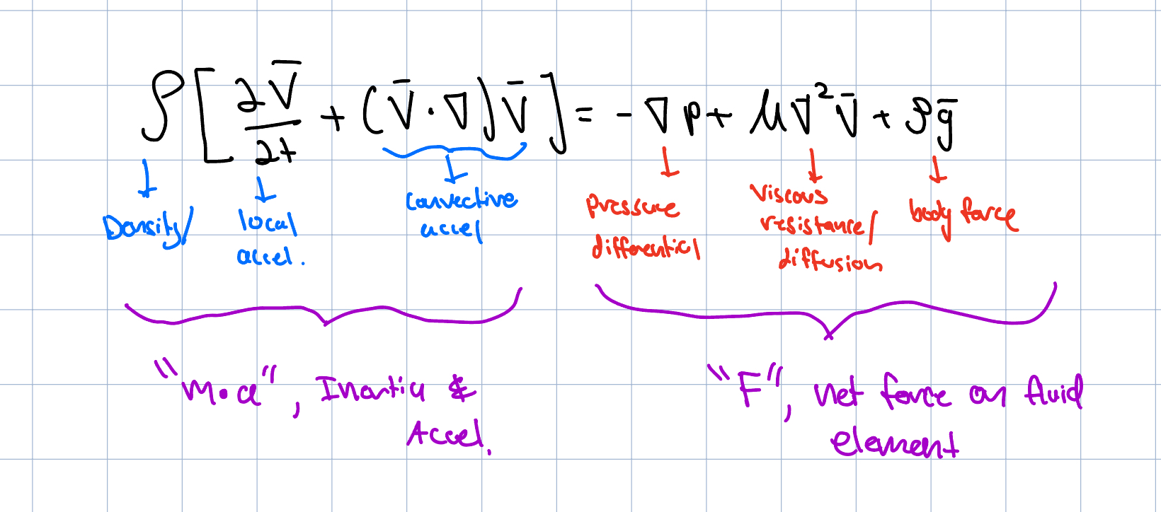
$$ \frac{D\vec{V}}{Dt} = \frac{\partial \vec{V}}{\partial t} + (\vec{V}\cdot\nabla)\vec{V} $$

the equations are often expressed as

$$ \rho \left[ \frac{\partial \vec{V}}{\partial t} + (\vec{V}\cdot\nabla)\vec{V} \right] = -\nabla p + \nabla \cdot \boldsymbol{\tau} + \rho \vec{g} $$

The left-hand side represents fluid acceleration, including both local and convective effects.

The terms on the right-hand side represent the forces acting on the fluid element:

$ (-\nabla p) $$-\nabla p$ corresponds to pressure forces
$ (\nabla \cdot \boldsymbol{\tau}) $ corresponds to viscous stresses
$ (\rho \vec{g}) $ corresponds to body forces such as gravity

These equations are generally coupled and nonlinear because the velocity components appear both directly and inside derivatives. Note that is pressure and viscous stress gradients and not raw values themselves that drive acceleration. It is also here that an earlier idea from The Big Idea of Fluid Mechanics reemerges, namely the key forces identified in Chapter 1. Here it is apparent that a proxy for inertia in density, when multiplied by acceleration, is exactly equal to the sum of forces acting on that differential fluid element. Again, this is nothing more than Newton's 2nd Law, a recurring motif in all of classical mechanics.

Cartesian Coordinates

When the momentum equations are expressed in Cartesian form they can be seen as

$$ \rho \left( \frac{\partial u}{\partial t} + u\frac{\partial u}{\partial x} + v\frac{\partial u}{\partial y} + w\frac{\partial u}{\partial z} \right) = -\frac{\partial p}{\partial x} + (\nabla \cdot \boldsymbol{\tau})_x + \rho g_x $$

$$ \rho \left( \frac{\partial v}{\partial t} + u\frac{\partial v}{\partial x} + v\frac{\partial v}{\partial y} + w\frac{\partial v}{\partial z} \right) = -\frac{\partial p}{\partial y} + (\nabla \cdot \boldsymbol{\tau})_y + \rho g_y $$

$$ \rho \left( \frac{\partial w}{\partial t} + u\frac{\partial w}{\partial x} + v\frac{\partial w}{\partial y} + w\frac{\partial w}{\partial z} \right) = -\frac{\partial p}{\partial z} + (\nabla \cdot \boldsymbol{\tau})_z + \rho g_z $$

These equations describe momentum conservation in the $x$-, $y$-, and $z$-directions.

Cylindrical Polar Coordinates

For many internal and rotating flows, cylindrical coordinates are more convenient.

The radial momentum equation is

$$ \rho \left( \frac{\partial V_r}{\partial t} + V_r\frac{\partial V_r}{\partial r} + \frac{V_\theta}{r} \frac{\partial V_r}{\partial \theta} - \frac{V_\theta^2}{r} + V_z\frac{\partial V_r}{\partial z} \right) = -\frac{\partial p}{\partial r} + (\nabla \cdot \boldsymbol{\tau})_r + \rho g_r $$

The tangential momentum equation is

$$ \rho \left( \frac{\partial V_\theta}{\partial t} + V_r\frac{\partial V_\theta}{\partial r} + \frac{V_\theta}{r} \frac{\partial V_\theta}{\partial \theta} + \frac{V_rV_\theta}{r} + V_z\frac{\partial V_\theta}{\partial z} \right) = -\frac{1}{r} \frac{\partial p}{\partial \theta} + (\nabla \cdot \boldsymbol{\tau})_\theta + \rho g_\theta $$

The axial momentum equation is

$$ \rho \left( \frac{\partial V_z}{\partial t} + V_r\frac{\partial V_z}{\partial r} + \frac{V_\theta}{r} \frac{\partial V_z}{\partial \theta} + V_z\frac{\partial V_z}{\partial z} \right) = -\frac{\partial p}{\partial z} + (\nabla \cdot \boldsymbol{\tau})_z + \rho g_z $$

These forms are commonly used in pipe flow, swirling flow, and axisymmetric flow analysis.

Euler Equations

If viscous effects are neglected, the stress terms vanish and the equations reduce to the Euler Equations:

$$ \rho \left[ \frac{\partial \vec{V}}{\partial t} + (\vec{V}\cdot\nabla)\vec{V} \right] = -\nabla p + \rho \vec{g} $$

These equations describe inviscid flow and are often useful when viscous effects are small compared to inertial forces. As we will see later, the ability to neglect such terms is often well-expressed in terms of non-dimensional quantities like the Reynolds number, which expresses the relative importance to inertial to viscous forces acting within a flow field. It should also be noted that the Bernoulli equation seen in chapter 3 can be achieved from direct integration of the Euler equations, connecting pressure, velocity and potential energy changes along a streamline.

Viscous Flow and the Navier--Stokes Equations

Real fluids experience viscous effects whenever velocity gradients are present. Viscosity produces internal friction within the fluid, causing momentum to diffuse through the flow field.

The general form of the momentum equation has already been presented, including viscous stresses. However, for Newtonian fluids, viscous stresses are proportional to velocity gradients. Substituting the Newtonian stress relationships into the differential equations of motion produces the well-known Navier--Stokes equations.

For incompressible flow with constant viscosity, the general vector form is

$$ \rho \left[ \frac{\partial \vec{V}}{\partial t} + (\vec{V}\cdot\nabla)\vec{V} \right] = -\nabla p + \mu \nabla^2 \vec{V} + \rho \vec{g} $$

Navier-Stokes intuitive analysis

The Navier--Stokes equations describe conservation of momentum for viscous fluid flow. The pressure gradient term drives the flow, the viscous term resists deformation through momentum diffusion, and the acceleration terms describe inertial effects. As stated before, because the equations contain nonlinear convective acceleration terms, exact analytical solutions are only possible for a limited number of simplified flows.

Cartesian Coordinates

The Cartesian Navier--Stokes equations are

$$ \rho \left( \frac{\partial u}{\partial t} + u\frac{\partial u}{\partial x} + v\frac{\partial u}{\partial y} + w\frac{\partial u}{\partial z} \right) = -\frac{\partial p}{\partial x} + \mu \left( \frac{\partial^2 u}{\partial x^2} + \frac{\partial^2 u}{\partial y^2} + \frac{\partial^2 u}{\partial z^2} \right) + \rho g_x $$

$$ \rho \left( \frac{\partial v}{\partial t} + u\frac{\partial v}{\partial x} + v\frac{\partial v}{\partial y} + w\frac{\partial v}{\partial z} \right) = -\frac{\partial p}{\partial y} + \mu \left( \frac{\partial^2 v}{\partial x^2} + \frac{\partial^2 v}{\partial y^2} + \frac{\partial^2 v}{\partial z^2} \right) + \rho g_y $$

$$ \rho \left( \frac{\partial w}{\partial t} + u\frac{\partial w}{\partial x} + v\frac{\partial w}{\partial y} + w\frac{\partial w}{\partial z} \right) = -\frac{\partial p}{\partial z} + \mu \left( \frac{\partial^2 w}{\partial x^2} + \frac{\partial^2 w}{\partial y^2} + \frac{\partial^2 w}{\partial z^2} \right) + \rho g_z $$

Cylindrical Polar Coordinates

In cylindrical coordinates, like before, the equations become more complex because the coordinate directions vary with position.

The radial Navier--Stokes equation is

$$ \rho \left( \frac{\partial V_r}{\partial t} + V_r\frac{\partial V_r}{\partial r} + \frac{V_\theta}{r} \frac{\partial V_r}{\partial \theta} - \frac{V_\theta^2}{r} + V_z\frac{\partial V_r}{\partial z} \right) = -\frac{\partial p}{\partial r} + \mu \nabla^2 V_r + \rho g_r $$

The tangential equation is

$$ \rho \left( \frac{\partial V_\theta}{\partial t} + V_r\frac{\partial V_\theta}{\partial r} + \frac{V_\theta}{r} \frac{\partial V_\theta}{\partial \theta} + \frac{V_rV_\theta}{r} + V_z\frac{\partial V_\theta}{\partial z} \right) = -\frac{1}{r} \frac{\partial p}{\partial \theta} + \mu \nabla^2 V_\theta + \rho g_\theta $$

The axial equation is

$$ \rho \left( \frac{\partial V_z}{\partial t} + V_r\frac{\partial V_z}{\partial r} + \frac{V_\theta}{r} \frac{\partial V_z}{\partial \theta} + V_z\frac{\partial V_z}{\partial z} \right) = -\frac{\partial p}{\partial z} + \mu \nabla^2 V_z + \rho g_z $$

These forms are widely used for internal flows and rotating fluid systems. It can be seen that in concert with the continuity equation, a system of partial differential equations is formed over four variables - the velocities in each coordinate direction and the pressure field. Still, the convective acceleration terms render these equations challenging to solve analytically, a caveat this pervasive in most flows. Still, a handful of analytical solutions are possible.

The No-Slip Condition

An extensive treatment of the Navier-Stokes equations is aided by knowledge in differential equaitons. That said, many will know that solving such equations requires boundary (and usually initial) conditions. A common boundary condition for viscous flows states that the fluid velocity at a solid surface matches the velocity of the surface itself. This behavior is known as the no-slip condition. Applying the no-slip boundary condition frequently appears when dealing with the Navier-Stokes equations, be it analytically or numerically.

For a stationary wall,

$$ \vec{V}=0 \qquad \text{at the wall} $$

while for a moving surface,

$$ \vec{V}=\vec{V}_{wall} \qquad \text{at the wall} $$

The no-slip condition produces velocity gradients near solid boundaries, which in turn generate viscous shear stresses within the fluid. This condition is responsible for the development of boundary layers and the characteristic velocity distributions observed in viscous internal flows such as pipe flow and flow between parallel plates.

Simple Laminar Flow Solutions

As mentioned already, the Navier--Stokes equations are difficult to solve in general, but several important analytical solutions exist for simple laminar flows. These solutions provide physical insight into how viscosity affects velocity distributions and wall shear stresses.

Flow Between Parallel Plates

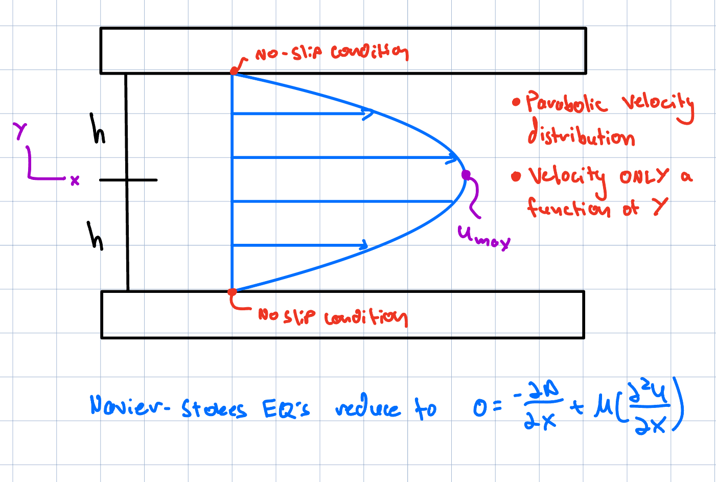
One classical solution involves steady, incompressible, fully developed flow between two stationary parallel plates separated by a distance $h$.

Under these assumptions:

velocity varies only in the transverse direction
pressure changes only along the flow direction
the flow is two-dimensional
inertial terms become negligible

The Navier--Stokes equations simplify significantly and produce the velocity profile

$$ u(y) = -\frac{1}{2\mu} \frac{dp}{dx} \, y(h-y) $$

The velocity is zero at the walls because of the no-slip condition and reaches a maximum midway between the plates. This parabolic profile demonstrates how viscous effects cause velocity gradients within the flow.

Visualization of flow between two infinite, flat plates

Laminar Pipe Flow

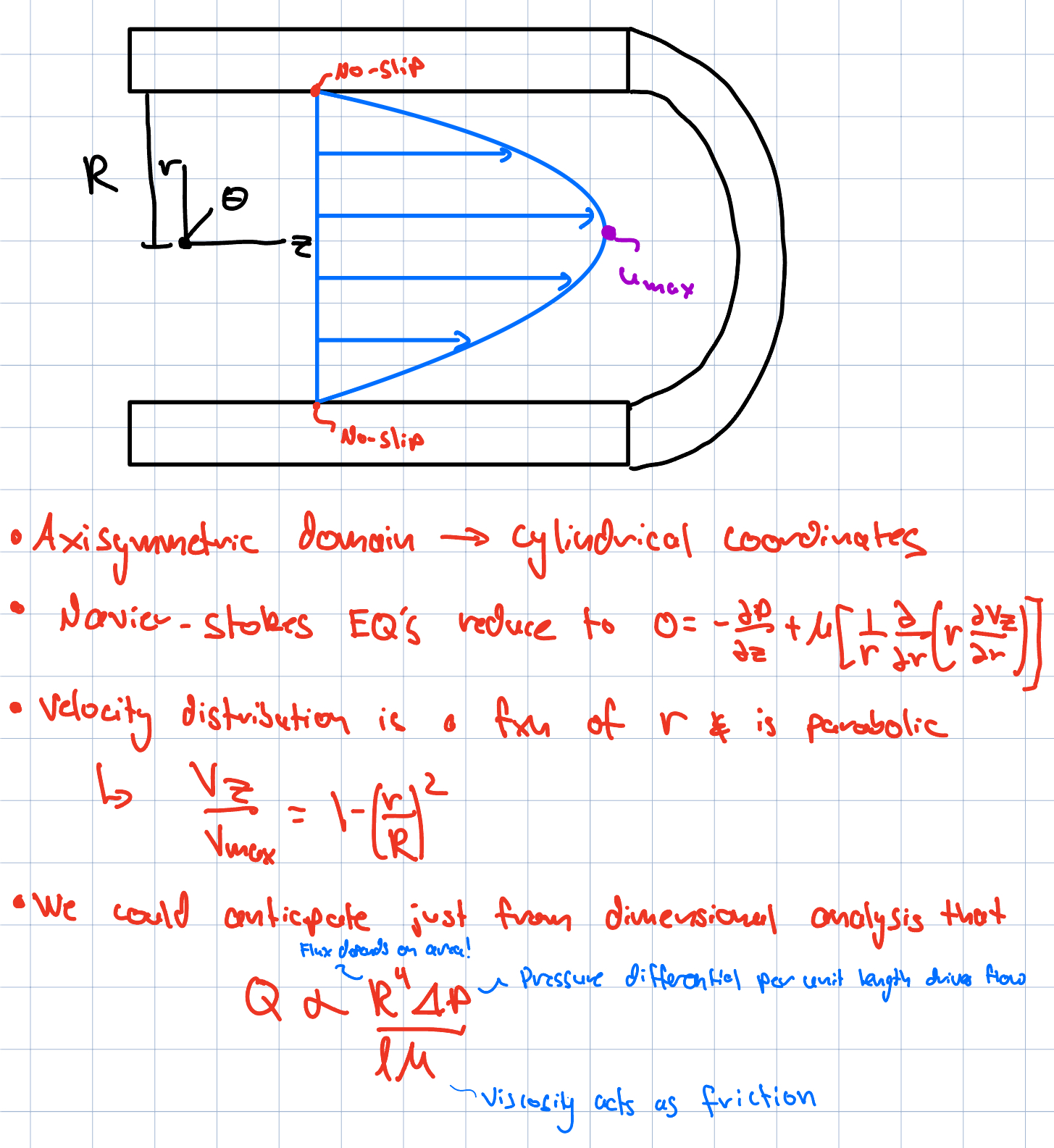
Another important analytical solution is steady, incompressible, fully developed flow through a circular pipe.

Under these assumptions, the velocity varies only with radial position, and the Navier--Stokes equations reduce to the Hagen--Poiseuille solution:

$$ u(r) = -\frac{1}{4\mu} \frac{dp}{dx} (R^2-r^2) $$

where $R$ is the pipe radius.

The velocity is maximum at the pipe centerline and decreases smoothly to zero at the wall because of viscous shear effects. Integrating the velocity profile over the pipe cross section gives the volumetric flow rate relationship

$$ Q = -\frac{\pi R^4}{8\mu} \frac{dp}{dx} $$

This relationship shows that pipe flow rate is highly sensitive to pipe radius because of the $R^4$ dependence.

These classical laminar flow solutions provide important physical insight into viscous fluid motion and serve as benchmark solutions for more advanced fluid mechanics analyses.

Visualization of analytic solution to laminar pipe flow

A Comment on Numerical Methods

It can be common for students to leave the treatment of differential fluid flow feeling as though it has few applications to real world flows given the difficulty in finding analytical solutions. Numerical methods resolves this by discretizing the flow domain and constructing linear algebraic equations that can be solved simaltaneously to approximate the Navier-Stokes equations. At a high level, by losing the continuous nature of the partial differential equation and solving only for values at a discrete set of points, partial derivatives can be approximated and transformed into linearized quantities. Many engineers will encounter and use these numerical methods implicitly through FEA (Finite Element Analysis) or CFD (Computational Fluid Dynamics) softwares. The softwares build are based on the governing partial differential equations for the domains that they solve over.