Introduction
Rolling bearings are a type of bearing that allows two components to move relative to each other using rolling elements. For example, a heavy slab moving on logs is a crude form of rolling bearings. With the invention of the Bessemer steel process in the mid 19th century, metal was able to be both smooth and hard, which allowed for bearings to be used more commonly.
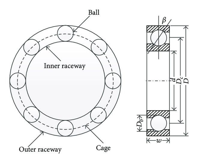
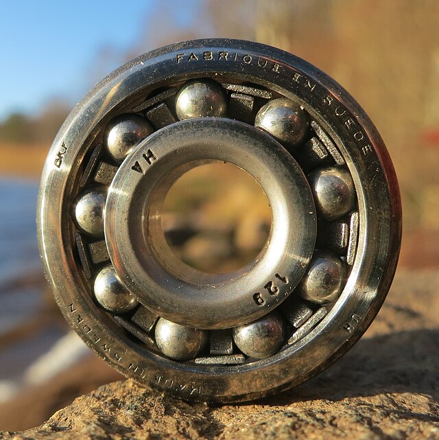
A rolling bearing consists of an inner race that is fixed to a shaft and an outer race that is fixed to a housing. In between the two races are the rolling elements, which lie in side grooves. The rolling elements can be different shapes, such as balls, cylinders, or barrel shaped. Rolling bearings are popular because they have very little friction, so they can start moving faster and can be used in many different conditions without much failure.
The rolling elements will always be in contact with both races as they lie in a groove. The forces and stresses at the contact can be determined from the maximum pressure, which is described by Hertz contact theory. The theory describes the stresses between curved, elastic bodies in contact. According to Hertz, the maximum pressure depends on the applied load, the curvature of the contacting surfaces, and the material properties of both bodies. Using these, the maximum contact pressure can be calculated, allowing engineers to predict stresses and design bearings that minimize wear and deformation.
where:
- F is the force applied
- E is the effective modulus of elasticity for two curved bodies
- R is the effective radius for two curved bodies
Bearing Life
Rolling bearings are subjected to cyclical stress and designed for a specific fatigue life. The formula for bearing life is given by the ratio:
where:
- \( L \) is the expected bearing life in revolutions.
- \( L_r \) is the reference life, \( 90 \times 10^6 \) revolutions for ball bearings.
- \( F_r \) is the applied radial load on the bearing.
- \( C \) is the rated load capacity, which is linked to \( L_R \) and represents the
This is the number of cycles that 90% percent of a group of identical bearings can endure under a constant radial load without the onset of surface fatigue.
constant radial load that a bearing can sustain for the reference life.
Rolling bearings experience cyclical stresses and can fail due to fatigue.
Impacts, load excursions, and shock loads increase stress, so a shock load factor \( K_a \) is used to account for these effects. Bearings are also analyzed statistically because their fatigue life varies across a set of identical components.
The distribution of bearing life is typically a Weibull distribution, which is asymmetric. The median life, or L50, is the point where 50% of bearings have failed. The L10 life corresponds to 90% reliability and is roughly 1/5th of the median. To account for reliability greater than 90%, a reliability factor Kr is applied.
Combining the effects of applied load, shock loading, and reliability, the modified equation for bearing life is:
where:
- \( K_a \) is the shock load factor, which accounts for impacts and load excursions.
- \( K_r \) is the reliability factor, which adjusts the life to meet a desired reliability level.
The shock load factor \( K_a \) and reliability factor \( K_r \) are selected based on the operating conditions and desired reliability of the bearing. A value of \( K_r = 1 \) corresponds to calculations performed with respect to the reference life, such as the \( L_{10} \) life (90\
Similarly, \( K_a = 1 \) represents low-shock or smooth operating conditions, while higher values of \( K_a \) account for increasing levels of impact or shock loading. For ball bearings, typical upper bounds for high-shock applications range up to approximately \( K_a = 3 \).
These parameter values are typically obtained from design charts and tables provided by bearing manufacturers or standards organizations, such as https://productselect.skf.com/\#/bearing-selection-start.
Angular Ball Bearings
The spherical rolling element bearings we have considered thus far are best for supporting radial loads. However, some components like helical or bevel gears also put a rotating shaft under axial or thrust loading. This changes the orientation of the stresses throughout the bearing, and reduces the life.
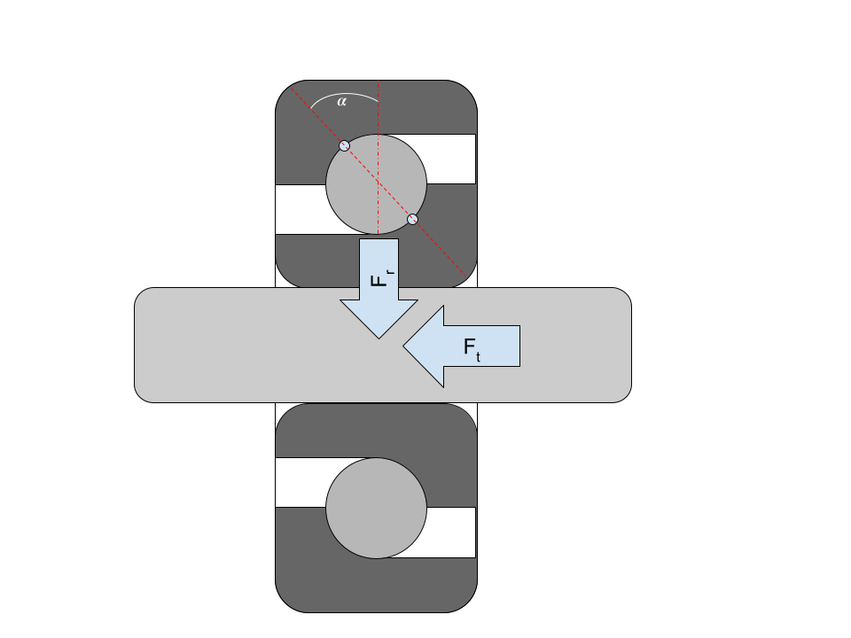
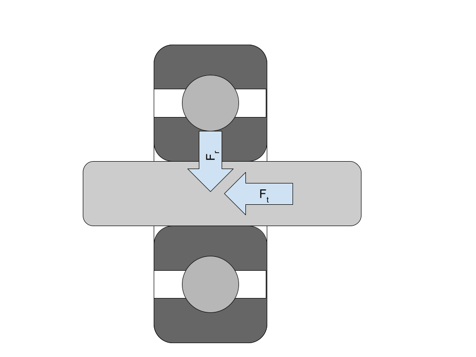
Angular ball bearings are better able to withstand thrust loads because races are cut asymmetrically to support the rolling elements further to one side. Statistical analysis of experimental data of bearing failures was used to identify an effective load \( {F_e} \) that can be used in place of Fr in predicting the life of a bearing, for both non-angular bearings (\( \alpha \)=0°) and angular bearings (\( \alpha \)=25°). These effective loads are based on the extent of the axial loading compared to radial loading, or \( {F_t} \)/\( {F_r} \). as seen in the table below.
| Bearing Type | Load Ratio Range | Effective Load \( F_e \)> |
|---|---|---|
| \( \alpha = 0^\circ \) | \( F_t/F_r < 0.35 \) | \( F_e = F_r \) |
| \( \alpha = 0^\circ \) | \( 0.35 < F_t/F_r < 10 \) | \( F_e = F_r \left[ 1 + 1.115 \left( \frac{F_t}{F_r} - 0.35 \right) \right] \) |
| \( \alpha = 0^\circ \) | \( F_t/F_r > 10 \) | \( F_e = 1.176\,F_t \) |
| \( \alpha = 25^\circ \) | \( 0.68 < F_t/F_r < 10 \) | \( F_e = F_r \left[ 1 + 0.870 \left( \frac{F_t}{F_r} - 0.68 \right) \right] \) |
| \( \alpha = 25^\circ \) | \( F_t/F_r > 10 \) | \( F_e = 1.176\,F_t \) |