Introduction
Many fluid mechanics problems involve flow around objects rather than through enclosed passages. This flow archetype is known as external flow. Examples include air moving around vehicles and aircraft, wind acting on buildings and bridges, and water flowing past ships, or submerged structures and objects. Perhaps the most popular instance of external people are familiar with is the idea of aerodynamics, which is nothing but external flow involving air as the working fluid.
When a fluid encounters an object, viscous effects near the surface alter the flow field and generate forces on the body. Depending on the flow conditions, these interactions may produce streamlined motion, separated wakes, pressure differences, and complex vortices.
This reference material examines the behavior of external flows and the forces generated by fluid motion around immersed bodies. As part of this study, boundary layer formation, drag, lift, flow separation, and the role of Reynolds number in determining flow behavior over these bodies will be explored.
Unlike many idealized inviscid flows, external flows are often strongly influenced by thin viscous regions near surfaces, even when the majority of the surrounding fluid behaves as if it were essentially inviscid. As one might expect from earlier chapters, fully analytic solutions to external flow problems are generally not possible. Thus, practical analysis frequently combines theoretical models, experiments, dimensional analysis, and empirical relationships. Many engineers will be familiar with applying Computational Fluid Dynamics (CFD) to external flow problems to solve them.

Overview of External Flow
External flow occurs whenever there is relative motion between a fluid and a solid body, whether fluid moves past a stationary object or the object moves through the fluid. It is common in external flow analysis to see physical bodies approximated as 2-D (extending to infinity in one coordinate direction) or axisymmetric shapes as opposed to an irregular 3-D profile. Similar to the simplifying assumptions of the Navier-Stokes equations in differential fluid flow, these approximations should be made judiciously. Overall, the behavior of external flows is strongly affected by viscosity, pressure distributions, and boundary layer development around the body.
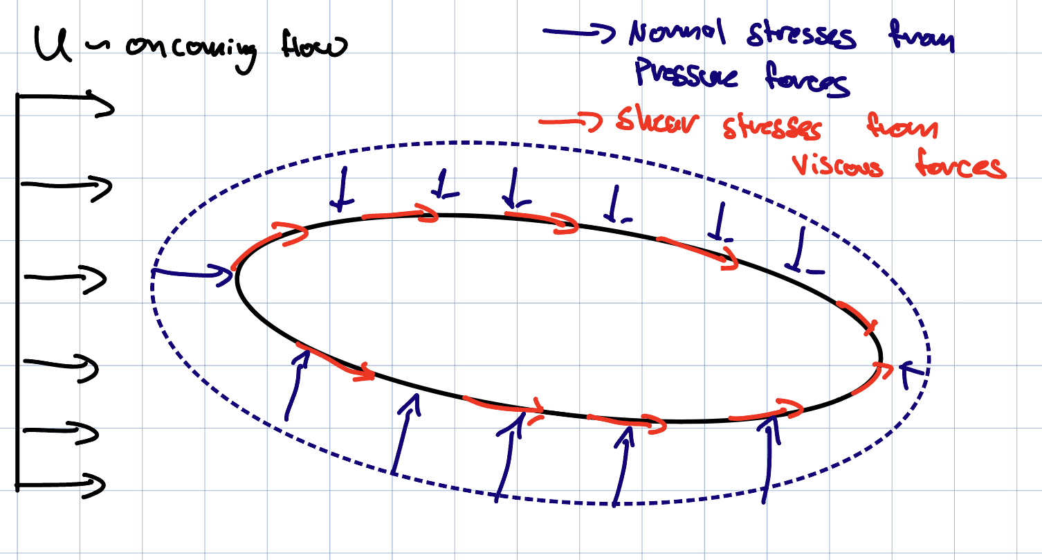
When fluid flows over an immersed body, pressure (acting normal to surfaces) and shear stresses (acting tangentially) develop along the surface of the object. These stresses produce net forces and moments that depend on the flow conditions and body geometry. For many external flow problems, the incoming flow far from the body may be approximated as a uniform free stream with velocity:
Pressure and Shear Forces
As stated, the fluid exerts both normal pressure forces and tangential shear forces on the surface of the body. The total aerodynamic or hydrodynamic force is obtained by integrating these surface stresses over the body.
In talking about the net effect of these forces, engineers usually consider drag force acts parallel to the incoming flow direction, while the lift force acts perpendicular to the free-stream velocity. Since it would be very difficult to know the pressure and viscous shear forces at each point along a body, it is impractical to attempt to integrate these contributions to identify the net force. Instead, these forces are commonly written in dimensionless form using drag and lift coefficients which are usually found through experiments:
- \( F_D \) is drag force,
- \( F_L \) is lift force,
- \( A \) is a reference area (usually taken as the projected area normal to oncoming flow).
Reynolds Number Effects
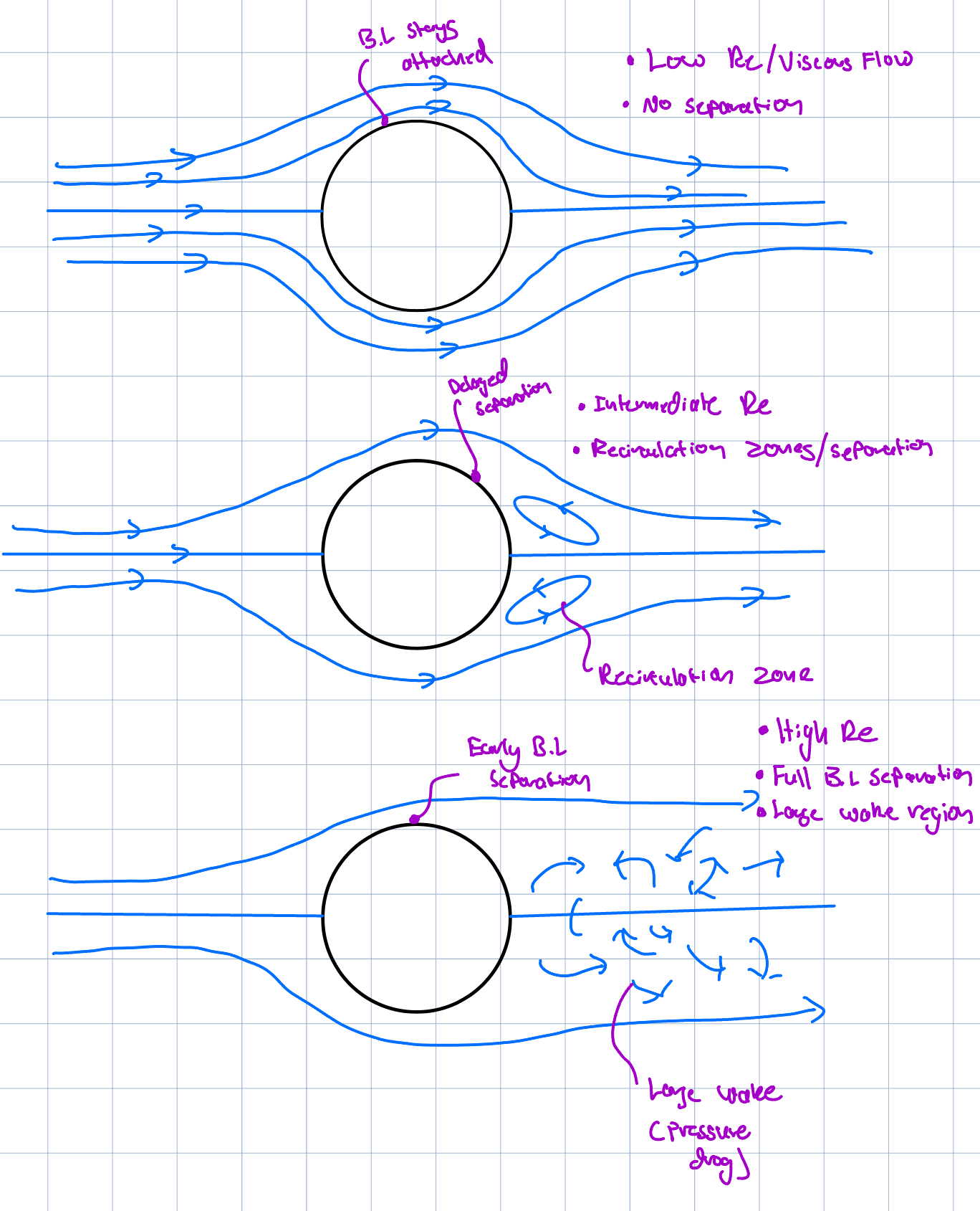
The structure of an external flow depends strongly on the Reynolds number:Boundary Layers and Wakes
Near the front of the body, fluid within the boundary layer initially follows the surface contour. Depending on the pressure distribution and flow conditions, the boundary layer may eventually separate from the surface. Flow separation produces a wake region downstream of the body that often contains recirculation, vortices, and increased energy dissipation. The size and structure of the wake strongly influence drag forces acting on the body. Streamlined bodies are designed to minimize wake formation and reduce drag, while blunt bodies generally produce larger separated regions and greater pressure losses.Boundary Layers
Although viscosity may only strongly influence a relatively thin region near a surface, this region plays a major role in determining drag, lift, and flow separation behavior. To be precise from the description above, boundary layer is the thin viscous region adjacent to a surface where fluid velocity changes from the no-slip condition at the wall to approximately the free-stream velocity farther away.Boundary Layer Development
As fluid moves over a surface, viscous effects diffuse momentum away from the wall and the boundary layer grows downstream from the leading edge. The boundary layer thickness is denoted by:Flow inside of boundary layers may remain laminar or become turbulent depending on the Reynolds number and surface conditions. Laminar boundary layers contain relatively ordered motion, while turbulent boundary layers contain fluctuating velocity components and enhanced momentum transport (flow and momentum is convected via bulk fluid motion compared to microscopic diffusive effects).
For flow over a smooth flat plate, transition often begins near:
.jpeg)
Displacement and Momentum Thickness
Since defining the boundary layer thickness using a fixed velocity percentage is somewhat arbitrary, other thickness measures are sometimes used. Because fluid velocity within the boundary layer is lower than the free-stream velocity, the boundary layer effectively reduces both the mass and momentum flux near the wall. The displacement thickness is nothing but the distance by which the body would need to be shifted outward to produce the same reduction in mass flow if no boundary layer existed at all:Blasius Flat Plate Solution
As alluded to above common external flow geometry for which more analytic methods and solutions have been developed is a flat plate. For laminar flow over a smooth flat plate with zero pressure gradient, the boundary layer equations admit an exact similarity solution known as the Blasius solution. Several important approximate relationships follow from this result.
The laminar boundary layer thickness is approximately:
is the Reynolds number based on distance from the leading edge.
The local wall shear stress is:
Boundary Layer Separation
As fluid flows along a surface, pressure changes within the outer flow can either accelerate or decelerate flow in the stramwise the boundary layer. If and when the flow encounters an adverse pressure gradient depending on its shape:
fluid near the wall may lose sufficient momentum that the boundary layer separates from the surface.
Again, separation often produces large wake regions, increased drag, and unsteady swirling or vortices downstream of the body. Streamlined bodies are therefore designed to delay separation and reduce wake formation whenever possible.
Drag
Drag is the component of fluid force acting parallel to the relative motion between a body and the surrounding fluid. In practical systems, drag is important because it determines quantities such as required propulsion power, fuel consumption, and overall aerodynamic or hydrodynamic efficiency.
Rather than attempting to directly integrate pressure and shear stresses over a complex surface, drag forces are commonly represented using the drag coefficient (repeated from above to clarity):
Pressure Drag and Skin-Friction Drag
Two primary mechanisms contribute to drag: skin friction and pressure drag.
Skin-friction drag results from viscous shear stresses generated within the boundary layer as fluid moves along the body surface. Bodies with large wetted (surrounded and influenced by fluid) surface areas may therefore experience significant friction drag even if flow separation is relatively small.
Pressure drag results from pressure differences between the upstream and downstream regions of the body. Large separated wake regions generally produce larger pressure drag because the pressure behind the body remains much lower than the pressure near the front stagnation region.
Streamlined and Blunt Bodies
The relative importance of pressure drag and skin-friction drag depends strongly on body geometry. Streamlined bodies are shaped to reduce separation and minimize wake size. Their drag is often dominated by skin-friction effects. Bluff bodies produce large separated wakes and correspondingly larger pressure differences between the front and rear surfaces. Their drag is therefore usually dominated by pressure drag.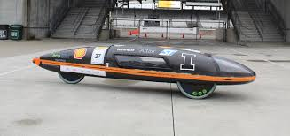
Reducing Drag
Many engineering designs attempt to reduce drag by either modifying boundary layer behavior or altering the overall body geometry.
One common strategy is to intentionally trigger transition to a turbulent boundary layer. Although turbulent boundary layers produce larger local shear stresses, they also contain greater momentum near the wall and are therefore more resistant to separation. In many cases, particularly at moderate to large Reynolds numbers, pressure drag brought on my separation is the more dominant contributor to overall drag.
A golf ball provides a well-known example of this effect. The dimples on the surface promote transition to a turbulent boundary layer, delaying flow separation farther downstream. This reduces the size of the wake region behind the ball and lowers pressure drag, allowing the golf ball to travel farther than a smooth sphere.
Another major method of reducing drag is to alter the body shape itself. Streamlined bodies are designed so the flow remains attached over a larger portion of the surface, minimizing wake formation and reducing pressure drag. In streamlined bodies, skin friction usually becomes a larger fraction of overall drag.
For example, an airfoil or teardrop-shaped body typically produces much smaller wake regions than a flat plate or blunt object of similar frontal area. As a result, streamlined bodies generally experience significantly lower drag coefficients.
Typical Drag Coefficients
Approximate drag coefficients for several common bodies are shown below. These are intended to be references for scale and basic shapes. Engineers should consult datasheets or experimental or numerical analysis to confirm the drag coefficient for their specific application.| Body Shape | Typical \( C_D \) |
|---|---|
| Streamlined airfoil | 0.04 -- 0.10 |
| Sphere | 0.1 -- 0.5 |
| Circular cylinder | 0.3 -- 1.2 |
| Flat plate normal to flow | 1.1 -- 2.0 |
| Cube | 0.8 -- 1.1 |
| Passenger automobile | 0.25 -- 0.4 |
Summary of Dependence of Drag Coefficient
As is probably clear at this point, the drag coefficient is dependent on many factors in complex ways. As usual, one of the most important is the Reynolds number:At relatively low Reynolds numbers, viscous effects strongly influence the entire flow field and drag coefficients are often comparatively large. As the Reynolds number increases, boundary layer transition and flow separation behavior may change significantly.
For some blunt bodies such as spheres and cylinders, transition to a turbulent boundary layer delays separation and reduces wake size, producing a sudden drop in drag coefficient known as the drag crisis.
In addition to Reynolds number, drag coefficients may also depend on:
- surface roughness,
- body orientation,
- compressibility effects,
- Mach number for high-speed flow.
Lift
Lift is the component of fluid force acting perpendicular to the relative flow direction. In many engineering systems, lift is intentionally generated to support loads, redirect flow, or extract energy from moving fluids. Common examples include aircraft wings, turbine blades, hydrofoils, and propellers.
Lift mostly results from pressure differences acting across the surface of a body. As fluid accelerates and decelerates around the geometry, the pressure distribution changes and a net force may develop.
Lift forces are commonly represented using the lift coefficient (repeated from above for clarity):
Again, similar to the drag coefficient,using a dimensionless coefficient allows lift measurements obtained from experiments or wind tunnel testing to be applied across geometrically similar systems.
Airfoils and Angle of Attack
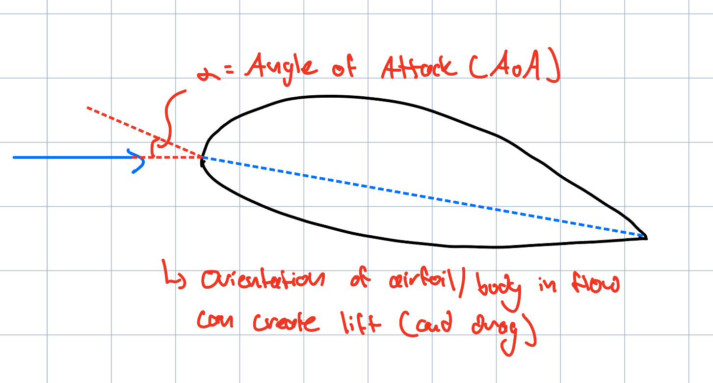
Many engineers will encounter lift in drag coefficients when dealing with or designing airfoils. Airfoils are specifically shaped to generate lift efficiently. In many cases, fluid velocity becomes larger over one surface of the body than the other, indicating pressure differences that generate a net force.
Lift generation depends strongly on angle of attack, which is the angle between the incoming flow direction and a characteristic reference line of the body. Increasing angle of attack generally increases pressure asymmetry around the body, producing larger lift forces. For small angles of attack, the lift coefficient for many airfoils varies approximately linearly with angle:
Boundary Layer Effects and Stall
Although lift is largely associated with pressure distributions, viscous effects remain extremely important because the boundary layer strongly affects flow attachment and separation. As angle of attack increases, the adverse pressure gradient over the upper surface becomes stronger. Eventually the boundary layer may separate from the surface, greatly altering the pressure distribution. Beyond a critical angle of attack, large-scale separation causes stall, which is characterized by:- rapid reduction in lift,
- increased drag,
- enlarged wake regions,
- unsteady flow structures.
Summary of Dependence of Lift Coefficient
In addition to the angle of attack as discussed above, lift coefficients are also influenced by Reynolds number because boundary layer behavior affects flow separation and pressure distributions around the body. At different Reynolds numbers, the location of transition and separation may shift, altering the resulting lift force.
Although this reference material focuses on incompressible flow, many engineers may encounter lift and drag coefficients when thinking about transonic or supersonic aviation. For compressible flows, Mach number becomes important as compressibility effects modify pressure distributions and shock formation may occur at high speeds.
Additional factors influencing lift coefficient include:
- airfoil camber,
- aspect ratio,
- surface roughness,
- wing sweep and geometry,
- flow unsteadiness.
Typical Lift Coefficients
Approximate lift coefficients for several common configurations are shown below. Actual values depend strongly on Reynolds number, angle of attack, surface roughness, and geometry.| Configuration | Typical \( C_L \) |
|---|---|
| Symmetric airfoil at \( 0^\circ \) AoA | \( \approx 0 \) |
| Cambered airfoil at small AoA | 0.3 -- 1.2 |
| High-lift wing with flaps | 1.5 -- 3.0 |
| Flat plate at small angle | 0.2 -- 0.8 |
| Circular cylinder with rotation | 0.2 -- 1.5 |
| Typical commercial aircraft wing | 0.5 -- 1.5 |
| Sail or hydrofoil | 0.5 -- 2.0 |