Introduction
At the end of the previous chapter, the Reynolds Transport Theorem was developed to relate system-based conservation laws to practical control volume formulations. In this chapter, those ideas are formalized and applied to the fundamental conservation equations used throughout fluid mechanics.
The chapter begins with conservation of mass and the continuity equation, which describe how mass is conserved as fluid flows through a control volume. Different forms of the continuity equation are developed for steady flow, incompressible flow, and one-dimensional approximations commonly used in engineering analysis.
The chapter then introduces the analogous formulation for linear momentum, applying RTT to reformulate Newton's 2nd Law to apply to control volumes. Much like traditional mechanics, applying these laws allows for the identification of unknown forces by connecting it to the kinematic behavior of fluid moving through a control volume.
After this, a final conservation equation, the energy equation, which applies the First Law of Thermodynamics to flowing fluids is developed for control volumes. This relationship accounts for changes in internal energy, kinetic energy, and potential energy while also incorporating work and heat transfer effects.
A number of examples will be provided for each of these conservation of principles to demonstrate their utility and show their connection tot he Reynolds Transport Theorem. Together, the conservation of mass, momentum and energy equations form some of the most important tools in fluid mechanics and are widely used in the analysis of pipes, pumps, turbines, nozzles, compressors, and many other engineering systems.
Mass Conservation and Continuity
Conservation of mass is one of the most fundamental principles in fluid mechanics. Regardless of how the fluid moves or deforms, mass cannot be created or destroyed. The continuity equation is therefore obtained by applying the Reynolds Transport Theorem to mass.
Using
in the Reynolds Transport Theorem gives
This equation states that any increase of mass inside the control volume must be balanced by a net inflow of mass, while any decrease in stored mass must correspond to a net outflow.
The first term,
represents accumulation or depletion of mass within the control volume.
The second term,
represents net mass flow across the control surface. The dot product with the outward normal vector ensures that outward flow contributes positively while inward flow contributes negatively.
The quantity
is often defined explicitly as the mass flow rate. For one-dimensional flow with approximately uniform properties across a section,
where \(V\) is the average velocity normal to the cross-sectional area.
Steady Flow Continuity Equation
For steady flow, no mass accumulates within the control volume:
and the continuity equation reduces to
For a single inlet and outlet,
If the flow is incompressible and density remains constant,
showing that velocity must increase when the flow area decreases. Recall that this is identical to the formulation that was stated in Chapter 3. Here, it has been derived using the Reynolds Transport Theorem.
When applying continuity, it is important to remember that velocity profiles are often nonuniform across real flow sections. In many engineering analyses, average velocities are used to simplify the equations.
Example: Basic Continuity Using RTT
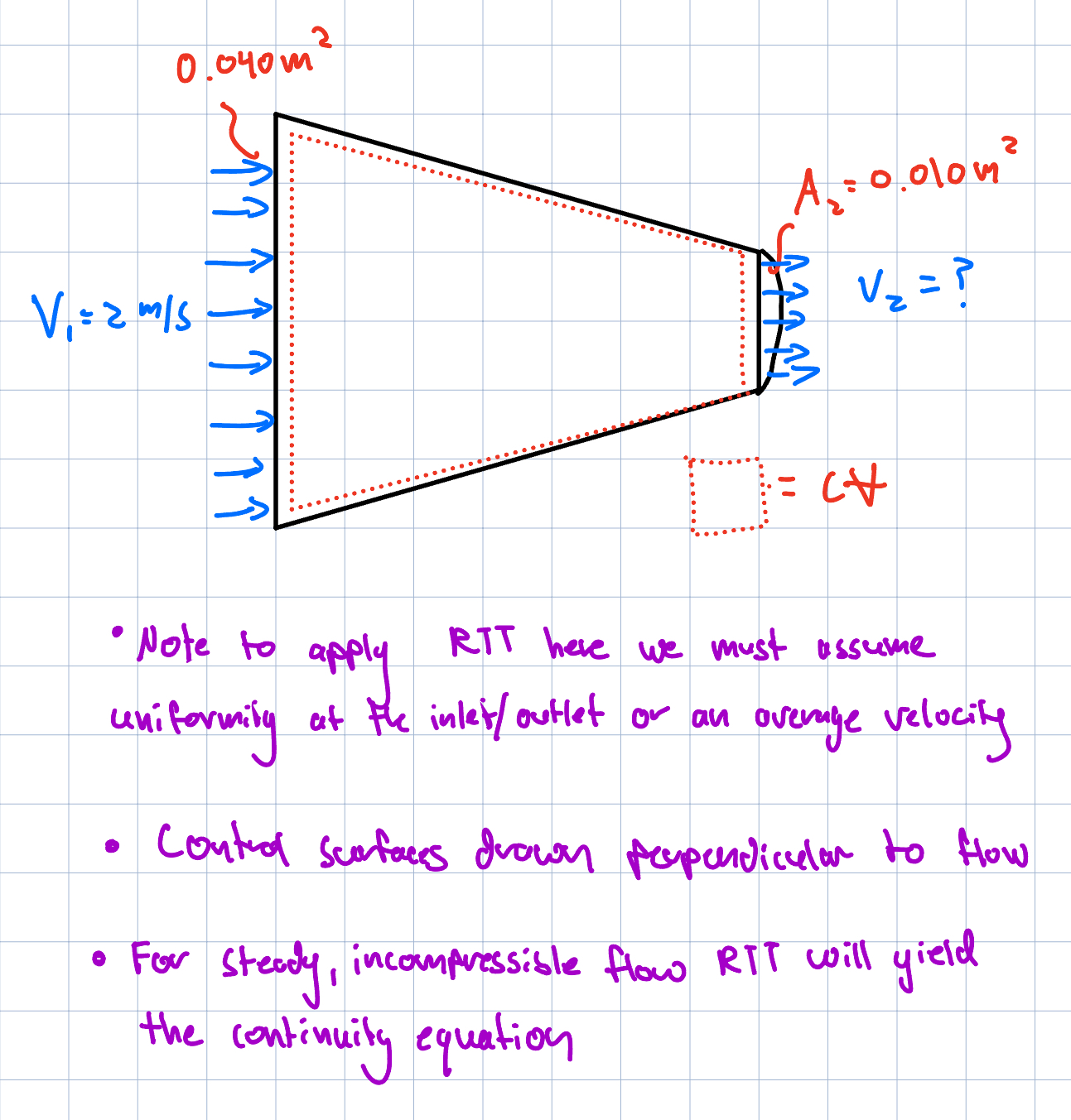
Consider steady incompressible flow through a converging duct. Water enters section 1 with area
and velocity
The duct narrows to
For mass conservation, apply RTT using \(B=m\) and \(b=1\):
For steady flow, the accumulation term is zero:
For one inlet and one outlet with uniform average velocity,
Therefore,
For incompressible flow, density cancels:
Solving for \(V_2\),
Substituting values,
The outlet velocity is larger because the same volume flow rate must pass through a smaller area.
Example: Continuity for an Angled Inlet
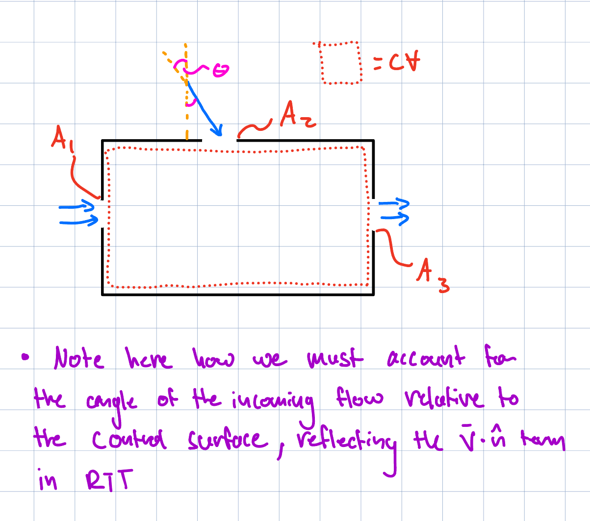
Consider a steady incompressible control volume with two inlets and one outlet. Inlet 1 enters horizontally with area \(A_1\) and velocity \(V_1\). Inlet 2 enters at an angle \(\theta\) relative to the outward normal direction of its control surface with area \(A_2\) and velocity \(V_2\). The flow exits through outlet 3 with area \(A_3\) and velocity \(V_3\).
Starting with the RTT form for conservation of mass,
For steady flow,
The mass flow crossing each control surface depends on the velocity component normal to the surface. Therefore, inlet 2 contributes
as its normal velocity component.
Using the sign convention that inflow is negative and outflow is positive,
Rearranging,
For incompressible flow, density cancels:
Solving for the outlet velocity,
This result shows that only the velocity component normal to the control surface contributes to mass flow through the surface.
Linear Momentum
The linear momentum equation is obtained by applying Newton's Second Law to a flowing fluid system. In fluid mechanics, the Reynolds Transport Theorem converts the system form of Newton's Second Law into a control volume formulation that is easier to apply to real engineering flows.
Linear momentum is a vector quantity defined as
Applying the Reynolds Transport Theorem using
gives
The left-hand side represents the total rate of momentum change associated with the control volume.
The first term,
corresponds to momentum accumulation within the control volume.
The second term,
represents net momentum transport across the control surface due to fluid motion.
The right-hand side represents the net external forces acting on the fluid. These forces may include
where:
- \( (\vec{F}_{pressure}) \) represents pressure forces acting on the control surface
- \( (\vec{F}_{body}) \) represents body forces such as gravity
- \( (\vec{F}_{shear}) \) represents viscous shear forces
- \( (\vec{F}_{external}) \) represents reaction or support forces
Since momentum is a vector quantity, the equation is generally applied separately in each coordinate direction.
Steady Flow Momentum Equation
For steady flow,
and the momentum equation reduces to
For one-dimensional flow with a single inlet and outlet and approximately uniform velocity profiles,
This relationship shows that forces arise whenever fluid momentum changes. Even if the speed remains constant, a change in flow direction still produces a force because momentum is directional. The momentum equation is widely used to analyze forces generated by flowing fluids, including aerodynamic drag, jet forces, and reaction loads on structures carrying fluid flow.
Example: Linear Momentum Using RTT
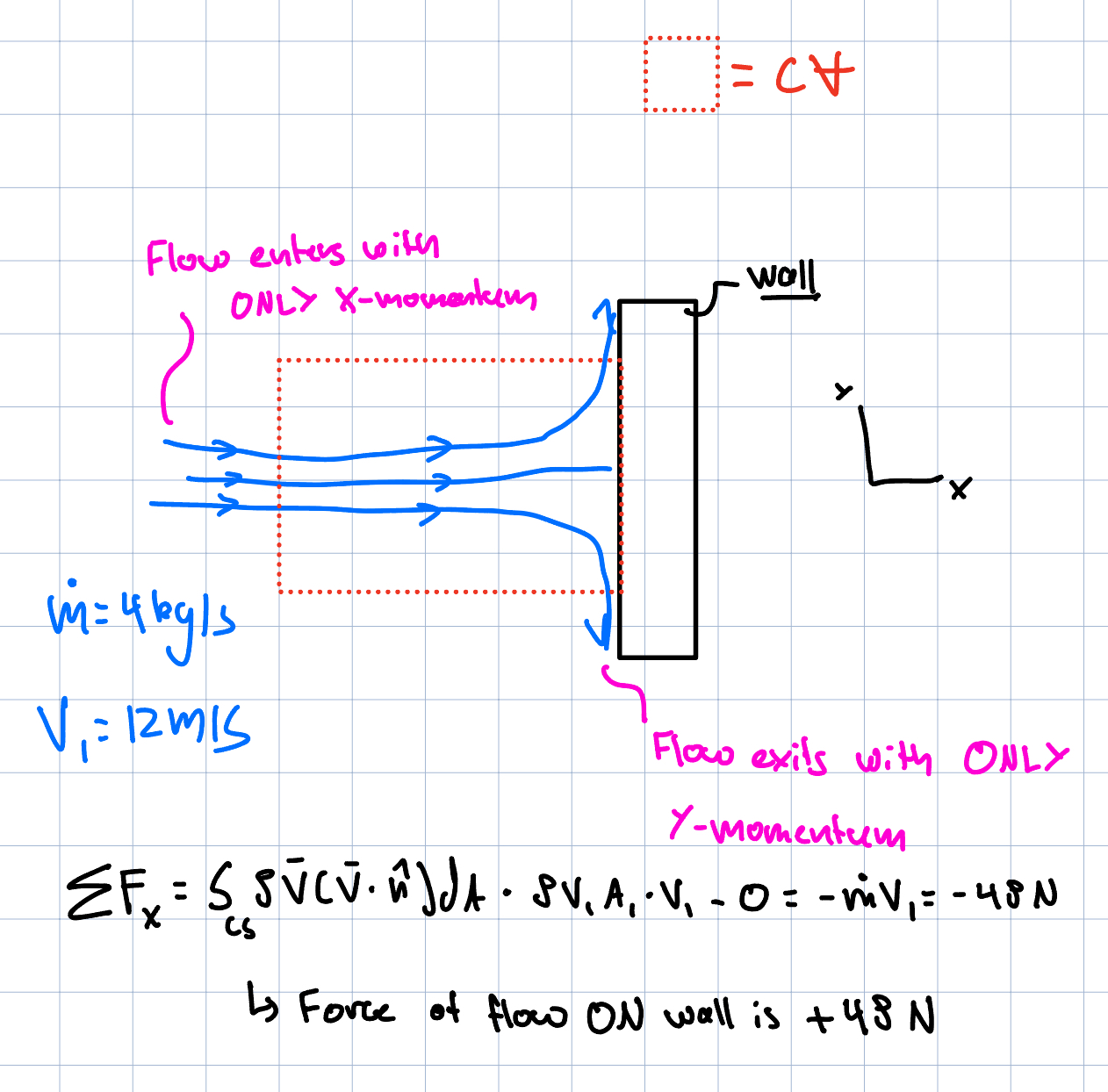
A horizontal water jet strikes a flat vertical plate and is brought to rest in the \(x\)-direction. The jet has mass flow rate
and inlet velocity
Apply RTT using \( (B=m\vec{V}) \) and \( (b=\vec{V}) \):
For steady flow, the accumulation term is zero:
For one-dimensional inlet and outlet flow,
The jet is stopped in the \(x\)-direction, so
Thus,
Substituting values,
Therefore, the plate exerts a force of
on the fluid. By Newton's Third Law, the fluid exerts an equal and opposite force on the plate:
in the positive \(x\)-direction.
Example: Moving Control Volume
A cart moves to the right with speed \(U\). A water jet also moves to the right with speed \(V\), where \(V>U\). The jet strikes a plate attached to the cart and is brought to rest relative to the moving plate. The jet area is \(A\), and the fluid density is \(\rho\). Find the force on the plate.
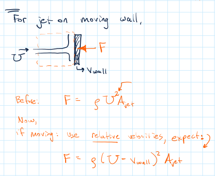
For a moving control volume, the flux term uses the relative velocity across the control surface:
Here,
The mass flow rate entering the moving control volume is therefore
In the moving frame of the plate, the incoming jet speed is \(V-U\), and it is brought to rest in the \(x\)-direction. Thus,
Substitute the relative mass flow rate:
This is the force of the plate on the fluid. Therefore, the force of the fluid on the moving plate is
Note the difference from the previous example. This force is smaller than the force on a stationary plate because the jet approaches the moving plate with a smaller relative speed.
The Energy Equation
The energy equation is obtained by applying conservation of energy to a flowing fluid system. In fluid mechanics, this equation accounts for the transport and conversion of different forms of energy as fluid moves through a control volume.
The total energy of a fluid includes:
- internal energy
- kinetic energy
- potential energy
Applying the Reynolds Transport Theorem together with the First Law of Thermodynamics gives the general control volume energy equation:
where:
- \( (\dot{Q}) \) is the rate of heat transfer into the control volume
- \( (\dot{W}) \) is the total rate of work done by the control volume
- \( (u) \) is the internal energy per unit mass
- \( (\frac{V^2}{2}) \) is the kinetic energy per unit mass
- \( (gz) \) is the potential energy per unit mass
The first integral term represents the rate of energy accumulation inside the control volume, while the surface integral accounts for energy transported across the control surface by fluid motion.
The work term \( (\dot{W}) \) includes both shaft work and flow work (pressure work). The flow work represents the energy required to push fluid across the control surface and is given per unit mass by:
Combining the flow work term with the internal energy gives the definition of enthalpy:
Using this substitution, the energy equation may be rewritten in enthalpy form as:
In this form, the pressure work has been absorbed into the transported energy term through the enthalpy \(h\).
Steady One-Dimensional Energy Equation
For steady flow with one inlet and one outlet and approximately uniform flow properties across each section, the energy equation reduces to
This form is commonly used in the analysis of pumps, turbines, compressors, heat exchangers, and many other engineering systems. Depending on the problem, certain terms may become negligible. For example, elevation effects may be small in horizontal flow systems, while kinetic energy changes may dominate in high-speed flows.
Mechanical Energy Equation
For incompressible flow, it is often convenient to express the energy equation in terms of mechanical energy per unit weight, or head. The mechanical energy equation is written as
where:
- \( (\frac{p}{\gamma}) \) is the pressure head
- \( (\frac{V^2}{2g}) \) is the velocity head
- \( (z) \) is the elevation head
- \( (h_A) \) is head added to the fluid
- \( (h_R) \) is head removed from the fluid
- \( (h_L) \) is head loss due to friction and irreversible effects
This equation describes how mechanical energy changes between two locations in a flow. Pumps increase the mechanical energy of the fluid, turbines remove energy from the flow, and viscous effects reduce usable mechanical energy through head losses.
Bernoulli's Equation
If the flow is frictionless and there are no pumps, turbines, or other energy interactions, the mechanical energy equation reduces to Bernoulli's Equation which was explored in Chapter 3. Again, along a streamline,
As was stated in Chapter 3, Bernoulli's Equation therefore represents conservation of mechanical energy for an ideal fluid flow, a special case of the general conservation approach developed here using the Reynolds Transport Theorem.
Example: Energy Equation for a Pump Up an Incline
Water is pumped from a lower reservoir to an upper reservoir. The elevation difference between the free surfaces is
The pump supplies
and the head loss in the pipe system is
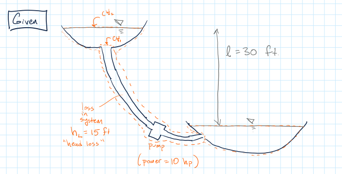
Choose a control volume around the pipe and pump, with the inlet at the lower reservoir free surface and the outlet at the upper reservoir free surface. At both free surfaces, the pressure is atmospheric, so
The reservoir surfaces are large, so the velocities are approximately zero:
Using the mechanical energy equation,
Canceling equal pressure terms and negligible velocity terms gives
Since
we get
The pump head added is related to shaft power by
Therefore,
Solving for \(Q\),
Substitute values. For water,
Also,
Thus,
The pump power is used to raise the water elevation and overcome the head loss in the pipe system.
Example: Pump Power Required
For the same reservoir-to-reservoir system, suppose the desired flow rate is \(Q\). Find the shaft power required to pump the fluid upward through an elevation difference \(\ell\) with head loss \(h_L\).
From the simplified mechanical energy equation,
The pump head is related to shaft power by
Therefore,
Solving for shaft power,
This expression shows that the required pump power increases with specific weight, flow rate, elevation rise, and head loss.