Introduction
Fluid mechanics is a branch of physics that studies the behavior and properties of liquids and gases, which may be either at rest or in motion. The behavior of fluids underlies phenomena that range from the flow of blood in arteries to flying aircraft to the raging waves and winds of hurricanes. The ubiquity of fluid systems in nature and everyday life make it necessary for engineers to become a proficient in designing and analyzing fluid systems. In the same vein, a robust foundation in fluid mechanics is essential for a number of adjacent fields in physics and mechanical engineering including thermodynamics and heat transfer. In total, by understanding how fluids respond to forces or interact with their surroundings, engineers are able to leverage them to create useful systems in fields like transportation, energy, environmental science and more.

These reference pages overview the core principles of fluid flow, specifically constant density or incompressible flow as is commonly covered in an introductory undergraduate engineering course. At the same time, these pages will provide a convenient bank of reference material, including equations, diagrams and charts that may be useful for a professional engineer working with a fluid system.
Defining a Fluid
The study of fluid mechanics necessarily begins with defining what actually qualifies as a fluid. In common terms, a fluid refers to both liquids and gases while excluding solids. Relative to solids, fluids contain comparatively weaker intermolecular forces and larger intermolecular spacing between their constituent molecules. Fluids are therefore easier to deform or compel to flow through interactions with their surroundings and containers.
This intuitive definition can be replaced by a more precise and useful definition of a fluid a follows:
A fluid is a substance which deforms continuously under the action of an applied shear stress, however small.
A shear stress is formed when a force acts tangent to or along the face of a surface. Under the effect of this stress, a solid generally deforms a finite amount whereas a fluid will continue to deform. In aggregate, this continuous deformation leads to the flow of a fluid or gas. While all fluids flow, the parameters of that flow can vary immensely depending on the properties of the fluid.
The Big Idea of Fluid Mechanics
When learning about fluids, it is essential to remember that most practical flows - which include most fluids and length and time scales an engineer could encounter - are governed by the same overarching physical laws as solids. Specifically, Newton's laws of motion, alongside the conservation of mass, momentum, and energy can be used to analyze or predict the behavior of entire fluid systems. In this way, learning about fluid mechanics is usually concerned with identifying the analogous forces and physical quantities for fluids as are used for solid mechanics.
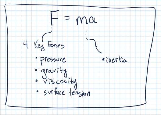
A good mnemonic that exemplifies this idea is the "Big Idea of Fluid Mechanics" as shown above. Most fluids problems can be solved by applying Newton's 2nd law. For fluids, one or a combination of four forces usually act on a fluid in an unbalanced manner to produce acceleration or they can balance to keep a fluid system static. These forces include, pressure, gravity, viscosity and surface tension. Such forces work to deform or accelerate a fluid in proportion to its inertia, its tendency to resist changes in motion. Inertia is represented in most equations in fluid mechanics with terms involving fluid density, \( \rho \) (analogous to the standard mass often found in for solid mechanics) and its velocity.
Pressure
Pressure is the force per unit area exerted by the fluid. It acts perpendicular to any surface in a fluid field (real or imaginary) and drives fluid motion from high to low pressure regions.

Gravity
Gravity is the body force acting on the fluid due to its mass. It is responsible for buoyancy and hydrostatic pressure, and is crucial in flows like rivers, oceans, or atmospheric phenomena.

Viscosity
Viscosity represents the internal friction of the fluid. It resists relative motion between fluid layers, dissipates kinetic energy as heat, and often determines whether a flow is laminar (highly smooth) or turbulent (chaotic).

Surface Tension
Surface tension arises from molecular forces at the interface of two immiscible fluids or a fluid and a solid. It acts to minimize surface area and governs droplet formation, capillary rise and many is usually important for fluid phenomena with small length scales.

Inertial vs Viscous Flows
The behavior of a fluid is usually dependent on whether the forces acting within the fluid system are primarily inertial or viscous in character. Inertia refers to a fluids' momentum and its tendency to resist changes in its motion. When a swimmer pushes through the water to propel themselves forward, they are able to do so because of the inertia of the fluid, its resistance to a change in momentum. By Newton's third law, an equal and opposite force is exerted on the swimmer and they move forward.
In contrast, imagine swirling a spoon through a thick syrup. Such a fluid can be called highly viscous; it is mainly difficult to move or flow because of the internal friction between adjacent layers of fluid, which limit relative motion as opposed to the inertia of the fluid.
Understanding when a flow is dominated by inertial or viscous forces can allow for simplifying assumptions or neglecting terms in governing fluid flow equations. As is covered in Module 5, there are quantitative ways to classify inertial and viscous flows such as using the Reynolds Number, but engineers should understand the qualitative differences in behavior between these two flow types.
Typical Unit Systems and Dimensions for Fluids Systems
As in any engineering calculation, it is important to understand the dimensions of a physical quantity, that is, the type of quantity that a given parameter or property is measuring. The fundamental dimensions are mass, length, time and temperature from other dimensions can be derived. Velocity for example has dimensions of length per unit time, a ratio between two fundamental dimensions.
Separately, engineers should be familiar with units, a standardized quantitative amount of a given physical quantity (a meter in length or a pound of mass as an example). Most fluid calculations are completed using the International System (SI), English Engineering (EE) or British Gravitational (BG) units. A valid physical equation should equate two quantities with the same physical dimensions and use a consistent set of units. The following table provides an overview of the dimensions and units for common fluid mechanics parameters. Helpful conversions can be found in Module 12.
| Quantity | Symbol | Dimensions | SI Units | English Units (EE / BG) |
|---|---|---|---|---|
| Length | \( L \) | \( [L] \) | m | ft |
| Time | \( t \) | \( [T] \) | s | s |
| Velocity | \( V \) | \( [L T^{-1}] \) | m/s | ft/s |
| Acceleration | \( a \) | \( [L T^{-2}] \) | m/s\( ^2 \) | ft/s\( ^2 \) |
| Force | \( F \) | \( [M L T^{-2}] \) | N | llbf |
| Mass | \( m \) | \( [M] \) | kg | lbm / slug |
| Density | \( \rho \) | \( [M L^{-3}] \) | kg/m\( ^3 \) | lbm/ft\( ^3 \) / slug/ft\( ^3 \) |
| Specific weight | \( \gamma \) | \( [M L^{-2} T^{-2}] \) | N/m\( ^3 \) | lbf/ft\( ^3 \) |
| Pressure | \( p \) | \( [M L^{-1} T^{-2}] \) | Pa (N/m\( ^2 \)) | lbf/ft\( ^2 \) (psf), psi |
| Dynamic viscosity | \( \mu \) | \( [M L^{-1} T^{-1}] \) | Pa\( \cdot \)s | lbm/(ft·s) |
| Kinematic viscosity | \( \nu \) | \( [L^2 T^{-1}] \) | m\( ^2 \)/s | ft\( ^2 \)/s |
| Surface tension | \( \sigma \) | \( [M T^{-2}] \) | N/m | lbf/ft |
| Bulk modulus | \( K \) | \( [M L^{-1} T^{-2}] \) | Pa | psi |
| Speed of sound | \( c \) | \( [L T^{-1}] \) | m/s | ft/s |
| Volumetric flow rate | \( Q \) | \( [L^3 T^{-1}] \) | m\( ^3 \)/s | ft\( ^3 \)/s |
| Mass flow rate | \( \dot{m} \) | \( [M T^{-1}] \) | kg/s | lbm/s |
| Energy | \( E \) | \( [M L^2 T^{-2}] \) | J | ft·lbf |
| Power | \( P \) | \( [M L^2 T^{-3}] \) | W | hp, ft·lbf/s |
Key fluid mechanics quantities with dimensions and units in SI and English (Engineering and British Gravitational) systems.
Magnitude References for Important Fluid Parameters
When analyzing a physical fluid system or interpreting results of an engineering simulation, it is very helpful to have an intuition for the magnitude of important quantities of a fluid. The following table provides one such reference to help build familiarity. The reynolds number, Re, is a dimensionless parameter used to classify fluid flow and is explained in Module 5.
| Flow Type | Velocity (m/s) | Length (m) | Density (kg/m\( ^3 \)) | Viscosity (Pa·s) | \( \boldsymbol{\Delta P} \)(Pa) | Re |
|---|---|---|---|---|---|---|
| Still air / natural convection | \( 10^{-4} \)\( 10^{-2} \) | \( 10^{-2} \)-\( 1 \) | \( \sim1 \) | \( 10^{-5} \) | \( 10^{-2} \)-\( 1 \) | \( <10^2 \) |
| Human-scale motion (walking, wind) | \( 0.1 \)-\( 10 \) | \( 1 \) | \( \sim1 \) | \( 10^{-5} \) | \( 1 \)-\( 10^2 \) | \( 10^4 \)-\( 10^6 \) |
| Vehicle aerodynamics (cars) | \( 10 \)-\( 40 \) | \( 1 \)-\( 5 \) | \( \sim1 \) | \( 10^{-5} \) | \( 10^2 \)-\( 10^3 \) | \( 10^6 \)-\( 10^7 \) |
| Aircraft (subsonic) | \( 100 \)-\( 300 \) | \( 10 \)-\( 50 \) | \( 0.3 \)-\( 1 \) | \( 10^{-5} \) | \( 10^3 \)-\( 10^4 \) | \( 10^7 \)-\( 10^8 \) |
| Pipe flow (water, household/industrial) | \( 0.1 \)-\( 3 \) | \( 10^{-2} \)-\( 1 \) | \( 0.3 \)-\( 1 \) | \( 10^{-3} \) | \( 10^2 \)-\( 10^5 \) | \( 10^3 \)-\( 10^5 \) |
| Microfluidics | \( 10^{-6} \)-\( 10^{-3} \) | \( 10^{-6} \)-\( 10^{-3} \) | \( 10^3 \) | \( 10^{-3} \) | \( 1 \)-\( 10^3 \) | \( 10^{-6} \)-\( 1 \) |
| Biological flow (blood in arteries) | \( 0.1 \)-\( 1 \) | \( 10^{-3} \)-\( 10^{-2} \) | \( \sim10^3 \) | \( 10^{-3} \) | \( 10^3 \)-\( 10^4 \) | \( 10^2 \)-\( 10^3 \) |
| Highly viscous flow (honey, oil) | \( 10^{-4} \)-\( 10^{-1} \) | \( 10^{-3} \)-\( 10^{-1} \) | \( 10^3 \)-\( 10^3 \) | \( 10^{-1} \)-\( 10^1 \) | \( 10^2 \)-\( 10^5 \) | \( <10 \) |
| Geophysical (rivers, atmosphere) | \( 0.1 \)-\( 10 \) | \( 10^1 \)-\( 10^6 \) | \( 1 \)-\( 10^3 \) | \( 10^{-5} \)-\( 10^{-3} \) | \( 10^2 \)-\( 10^5 \) | \( 10^6 \)-\( 10^{10} \) |
Order-of-magnitude ranges for fluid flows, including characteristic driving pressure differences \( \Delta P \) and dynamic pressure \( \frac{1}{2}\rho V^2 \).
Caution in Analyzing Dimensions
Some physical quantities may have the same dimensions, this does not mean they measure the same quantity. Nevertheless, dimensions and units provide insight into how a physical quantity is defined and how it is relevant for a fluid system. Dimensions are also important for dimensional analysis, which is covered in Module 10.
As an example, both pressure (\( p \)) and energy density (\( u \)) have the same physical dimensions, but they represent different physical concepts.
Pressure is defined as force per unit area:
Dimensionally, this is
Energy density conversely is energy per unit volume:
Dimensionally, this is
Although \( [p] = [u] = M L^{-1} T^{-2} \), pressure describes a force distributed over an area, while energy density describes energy stored per unit volume. They are dimensionally equivalent but physically distinct quantities
Assuming Incompressibility
Introductory fluid mechanics is typically taught with the overriding assumption that the working fluid is incompressible, that is, its density (or specific volume), is constant.
As was already discussed, density is a proxy for the inertia of a fluid. For most common liquids, most notably water, the density of the fluid is a weak function of temperature and pressure. As a result, over a wide range of engineering conditions the density of liquids can be assumed to be constant without incurring significant error in calculations.
In contrast, the density of a gas is strongly influenced by variations in pressure and temperature. However, it can be shown that incompressibility can be assumed for gases as well so long as its Mach number, that is, the speed of the fluid relative to the local speed of sound, is not too high.
For most gases, a good rule of thumb is that if the gas has a Mach number of less than about 0.3 (traveling at 30\
While all real fluids are compressible to some degree, the assumption of incompressibility is useful for many fluids problems because it simplifies the governing fluids equations and makes many fluids problems tractable. As a preemptive example, consider the general conservation of mass equation for a fluid which is covered in greater detail in Module 5.
Starting from the compressible form:
Assuming \( \rho = \text{constant} \):
Thus:
Since \( \rho \neq 0 \):
Treating a fluid as incompressible eliminates the time-dependent term,
and simplifies the adjective term
to create a first order partial differential equation in space only.
Even without knowing the precise derivation or applications of this equation, it is clear that its final form for an incompressible fluid has been simplified. In almost all cases, incompressible flow makes such equations easier to apply and solve analytically or numerically.
An engineer should always use good judgment to understand if the assumption of incompressibility is still valid for a given working fluid, considering the changes in pressure or temperature that fluid experiences. Error in calculations due to ignoring compressibility are generally nonlinear and can produce noticeable errors for mostly gaseous and high-speed systems if not accounted for. It is also important to recall that most of the equations and concepts presented in these reference pages assume incompressibility by default. Indeed compressible fluids often exhibit behaviors that are different or even exactly opposite that of their incompressible counterparts.