Current page:

Introduction

In conjunction with fluid statics, the second essential domain of fluid mechanics is that of dynamics. Again, invoking The Big Idea of Fluid Mechanics from chapter 1, dynamic fluid situations are those in which forces acting on a fluid produce acceleration, that is, the change in velocity of fluid particles. In general, dynamic flows may be driven by a combination of the forces outlined in The Big Idea; however, the simplest and largest category of flows are those driven primarily by gravity and pressure forces. For these flows, the viscosity of a fluid, which is primarily responsible for shear stresses present in a flow, can be neglected (inviscid flow). Critically, dynamic fluids are governed by Newton's laws and therefore, the fluid flow equations derived to describe them represent familiar laws from other areas of mechanics: conservation of mass, momentum and energy.

Streamlines

When describing the motion of a moving or dynamic fluid, the main thrust is to apply Newton's 2nd Law to a fluid particle, such that forces can be related to changes in a particle's direction and speed. For fluids, a convenient coordinate system to do this is the tangent-normal coordinate system, wherein one coordinate direction is oriented along the current direction a particle is traveling (along its current velocity vector), and another perpendicular to this path pointing in the direction of curvature.

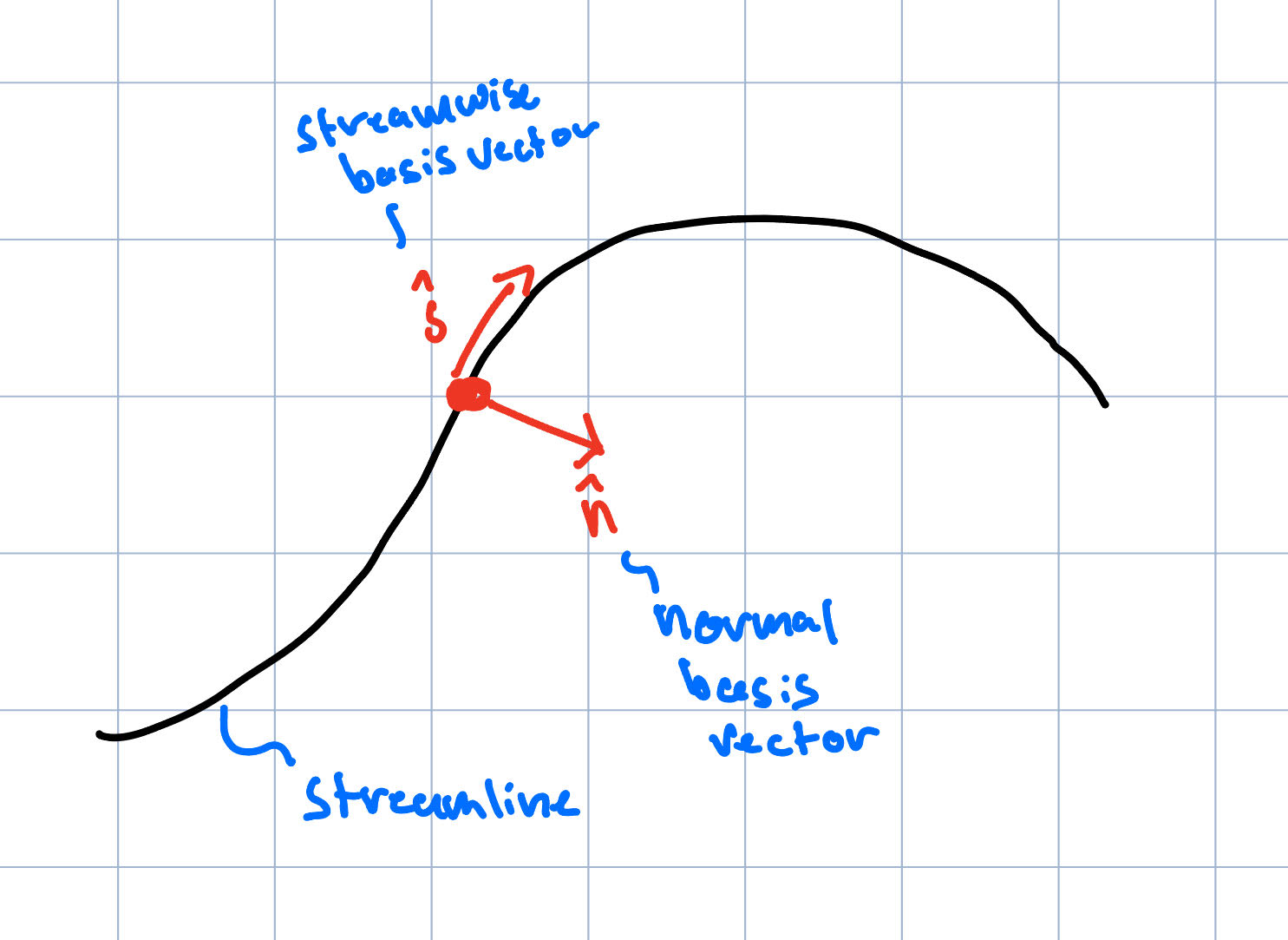
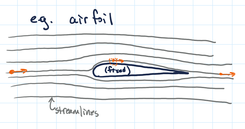
Tangent (Streamwise - Normal Coordinate representation of a Fluid Particle

As a particle flows through time and space, it traces a given path in time and space. This imaginary path is known as a streamline. It represents a history of the position of a particle through time and therefore is tangent to the velocity vector of that particle at every moment in time. If a flow is known to be steady, then there is no change in velocity (or any other flow property) at a given point in space across time. Physically, this means that the streamlines do not change in time and successive fluid particles that began at the same position follow the same path. In a full flow, one could imagine many streamlines, each of which may have their own shapes and directions, that define the overall movement of the entire flow.

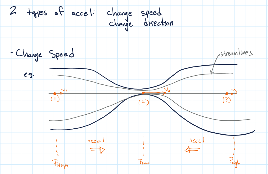
Streamlines of air passing over an airfoil

For a steady flow, the acceleration of a particle along a streamline can occur along a streamline (change speed), or normal to a streamline (change direction) and can be expressed thusly:

$$ \text{Streamwise acceleration:} \quad a_t = V \frac{dV}{ds} $$

$$ \text{Normal acceleration:} \quad a_n = \frac{V^2}{R} $$

$ V $ = fluid speed (magnitude of the velocity), scalar
$ \vec{V} $ = velocity vector, tangent to the streamline
$ s $ = distance along the streamline, scalar coordinate
$ R $ = radius of curvature of the streamline
$ a_t $ = tangential acceleration, along the streamline
$ a_n $ = normal acceleration, directed toward the center of curvature

With an acceleration adequately defined for a fluid particle, a general force balance results in the equation of motion for steady, non-viscous flow.

$$ \text{Along a streamline:} \quad \gamma \sin\theta - \frac{\partial p}{\partial s} = \rho V \frac{\partial V}{\partial s} $$

$$ \text{Normal to a streamline:} \quad - \rho g \frac{dz}{dn} - \frac{\partial p}{\partial n} = \rho \frac{V^2}{R} $$

$ \vec{V} $ = velocity vector (tangent to streamline)
$ V $ = fluid speed (magnitude of $ \vec{V} $)
$ s $ = coordinate along the streamline
$ n $ = coordinate normal to the streamline
$ p $ = pressure
$ \rho $ = fluid density
$ \gamma = \rho g $ = specific weight
$ g $ = gravitational acceleration
$ z $ = elevation (vertical coordinate)
$ \theta $ = angle of streamline relative to the horizontal
$ R $ = radius of curvature of the streamline

These equations, which include partial derivatives and a streamwise coordinates are nothing for than an expression of Newton's 2nd Law, F = ma. For each equation, the first term on the left represents the force of gravity acting along that coordinate direction and the second the pressure force (it enters as a derivative since spatial changes in pressure result in net forces). The terms make up the sum of the forces acting on the particle. The term on the right is exactly the acceleration of the particle in the given coordinate direction. In total, an imbalance of pressure and gravity forces produces acceleration of a fluid still assuming steady, non-viscous flow. For fluids, the size of forces is often extensive, that is, proportional to the amount of fluid present. As a result, it is density, not mass, that appears to represent inertia in many fluid dynamics equations.

The Bernoulli Equation

In principle, the above equations are sufficient to describe the acceleration and resulting kinematics of a steady, inviscid, incompressible fluid flow, relating pressure and gravity to acceleration. However, a more useful form can be arrived at by integrating these equations. Doing so results in a more amenable set of expressions:

$$ \text{Along a streamline:} \qquad \int \frac{dp}{\rho} + \frac{V^2}{2} + gz = Constant $$

$$ \text{Normal to a streamline:} \qquad \int \frac{dp}{\rho} + gz + \int \frac{V^2}{R}\,dn = Constant $$

Where C represents a constant that is established by the nature of the flow somewhere along the streamline. Assuming incompressibility (constant density), these equations can be further simplified in a form that is easy to apply to fluid problems.

$$ \text{Along a streamline (incompressible):} \qquad {p} + \frac{\rho V^2}{2} + \rho gz = Constant $$

$$ \text{Normal to a streamline:} \qquad p + gz + \int \frac{V^2}{R}\,dn = Constant $$

The first of these equations is the famed Bernoulli Equation Which is sometimes rewritten explicitly to relate points along the same streamline.

$$ \text{Point 1} \quad {p_1} + \frac{\rho V_1^2}{2} + g z_1 = {p_2} + \frac{\rho V_2^2}{2} + g z_2 \quad \text{Point 2} $$

Together, these equations can be used to identify and solve for flow conditions (velocity, pressures and vertical displacement), at a given point along a streamline provided sufficient information is available at a separate point in the streamwise or normal direction Recall that these equations have been derived under and are only valid with the following assumptions.

Steady flow: Flow properties do not change with time at a given point
Inviscid flow: Viscous effects (friction) are negligible
Incompressible flow: Density $ \rho $ is constant
Along a streamline: Equations are applied along a single streamline
No energy addition/removal: No pumps, turbines, or heat transfer
Gravity is the only body force: Other body forces are neglected

Note that in the form of the Bernoulli equation presented here, the dimensions of the terms are the same as those of pressure, however, many other forms are possible by normalizing by various terms in the equation. For instance, dividing the equation by the specific weight for instance, produces terms with dimensions of length, that is, pressure head.

Interpreting the Bernoulli Equation

So far, it has been shown that the Bernoulli Equation can be arrived at by integrating Newton's 2nd Law along a streamline and enforcing certain assumptions about the nature of flow. Note that even in its integrated form, the Bernoulli equation relates the forces due to gravity and pressure ( $ \rho gz $ and $ p $) to a term reminiscent of acceleration ($ \frac{\rho V^2}{2} $). That said, by integrating the equations of motion for a fluid particle, the resulting Bernoulli Equation is a statement of conservation of energy. Flow work done by changes in pressure or changes in gravitational potential energy must be accounted for by corresponding changes in the kinetic energy of the fluid.

Static, Dynamic, and Total Pressure

This energy interpretation of Bernoulli’s equation is often expressed in terms of different ``types'' of pressure. Each term in the equation corresponds to a distinct contribution to the fluid’s mechanical energy per unit volume (equivalent dimensions to the dimensions of pressure).

The static pressure $ p $ represents the thermodynamic pressure of the fluid. It is the pressure that would be measured by a probe moving with the flow and is associated with the fluid’s internal energy and its ability to do flow work.

The dynamic pressure is defined as

$$ q = \frac{1}{2}\rho V^2 $$

and represents the kinetic energy of the fluid due to its motion. It can be interpreted as the pressure rise that would occur if the fluid were brought to rest without losses.

Combining these gives the total (or stagnation) pressure:

$$ p_0 = p + \frac{1}{2}\rho V^2 $$

which represents the total mechanical energy of the flow per unit volume (excluding elevation effects).

In flows where elevation changes are negligible, Bernoulli’s equation reduces to

$$ p + \frac{1}{2}\rho V^2 = \text{constant} $$

showing that an increase in velocity must be accompanied by a decrease in static pressure, and vice versa, in order to conserve energy along a streamline.

Using the Bernoulli Equation

Most of the time, engineers use the Bernoulli equation to solve problems by relating two points along the same streamline. Their interest is in solving for the velocity or pressure of a flow at point somewhere downstream and not the actual value of the constant preserved along the streamline. By writing the equation between two flow points, unknown quantities such as pressure or velocity can be solved using known conditions elsewhere in the flow.

In practice, the equation is often simplified by choosing convenient reference points. For example:

Elevation $ z $ can be set to zero at a chosen datum.
Pressure terms may cancel if both points are exposed to the same atmospheric pressure.
Velocity at large reservoirs is often approximated as $ V \approx 0 $.

These simplifications reduce the equation while preserving the underlying energy balance, but they must be justified based on the physical situation.

Conservation of Mass (Continuity)

The conservation of mass states that mass cannot be created or destroyed within a flow. For a control volume, this requires that the mass flow rate entering equals the mass flow rate leaving (for steady flow).

Mass flow rate

$$ \dot{m} = \rho A V $$

where $ \rho $ is density, $ A $ is cross-sectional area, and $ V $ is the average velocity normal to the area.

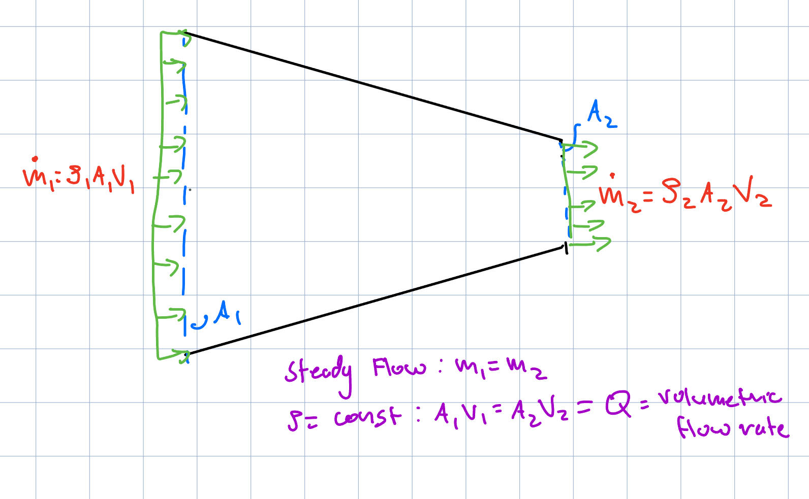
Conservation of Mass and Basic Continuity

Continuity equation (steady flow)

$$ \dot{m}_{in} = \dot{m}_{out} $$

For a single inlet and outlet:

$$ \rho_1 A_1 V_1 = \rho_2 A_2 V_2 $$

Incompressible flow

If density is constant, the equation simplifies to

$$ A_1 V_1 = A_2 V_2 $$

This shows that a decrease in area must result in an increase in velocity.

Connection to Bernoulli

Continuity and Bernoulli are used together to solve flow problems:

Continuity relates velocity and area
Bernoulli relates velocity and pressure

Together, they allow determination of unknown pressures, velocities, or flow rates in systems such as nozzles, pipes, and measurement devices.

Bernoulli Phenomena

Bernoulli’s equation explains many common fluid flow devices and phenomena by relating changes in pressure to changes in velocity and elevation. The following are standard applications.

Venturi Tube

A Venturi tube consists of a converging section, a throat, and a diverging section. As the flow enters the throat, the area decreases, causing the velocity to increase and the pressure to decrease.

Venturi Tube: flow is faster in narrow sections and slower in fatter sections

Applying continuity and Bernoulli between section's 1 and 2:

$$ A_1 V_1 = A_2 V_2 $$

$$ p_1 + \frac{1}{2}\rho V_1^2 = p_2 + \frac{1}{2}\rho V_2^2 $$

Solving for flow velocity using the pressure difference:

$$ V_2 = \sqrt{ \frac{2(p_1 - p_2)}{\rho \left(1 - \left(\frac{A_2}{A_1}\right)^2 \right)} } $$

A typical Venturi tube will have a static pressure tap or another pressure-measuring device at the wide and thin section*s of the tube which can be used along with the cross-section*al areas to quantify the flow velocities.

Pitot Tube

A Pitot tube measures flow velocity by bringing the fluid to rest at a stagnation point.

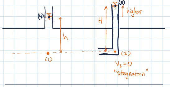
Measuring static and stagnation pressure with a Pitot tube

Applying Bernoulli between the free stream and the stagnation point:

$$ p_0 = p + \frac{1}{2}\rho V^2 $$

Solving for velocity:

$$ V = \sqrt{ \frac{2(p_0 - p)}{\rho} } $$

where $ p_0 $ is the stagnation pressure and $ p $ is the static pressure. Overall, this device permits an accurate estimation of velocity based off of measured pressures from a flow field. Pitot tubes are commonly employed on airplanes to assess airspeed.

Free Jet from a Tank

For a fluid exiting a tank through a small opening, the velocity of the jet can be found using Bernoulli between the free surface and the exit point.

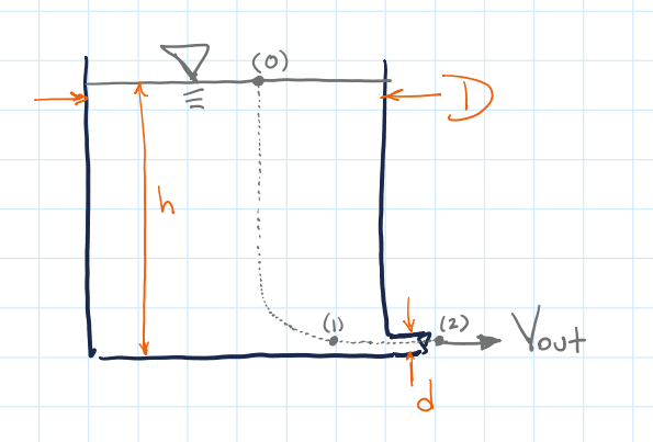
A large reservoir ejecting fluid for a narrow outlet at the bottom. A Bernoulli streamline can be charted from the top surface with essentially zero velocity to the faster moving being propelled out at the bottom

Assuming both points are exposed to atmospheric pressure and the surface velocity is negligible:

$$ V = \sqrt{2g(h_0 - h_2)} $$

If the free surface is taken as the reference elevation:

$$ V = \sqrt{2gh} $$

This result is known as Torricelli’s law, and it shows that the exit velocity depends only on the height of the fluid above the opening.

These three examples demonstrate the working exchange of flow work, gravitational potential energy and kinetic energy described by the Bernoulli equation.

Increased velocity $ \rightarrow $ decreased static pressure (Venturi)
Flow brought to rest $ \rightarrow $ maximum pressure (Pitot)
Potential energy $ \rightarrow $ kinetic energy (free jet)

Limitations of the Bernoulli Equation

The Bernoulli equation is derived under several aforementioned assumptions. To reiterate, these are that the flow under consideration be incompressible, steady, inviscid and along a streamline. When these assumptions are violated, the Bernoulli equation is no longer accurate and cannot be used or must be modified as will be seen in later chapters. One of the most common errors in fluid dynamics is the overuse of the Bernoulli equation to describe flows for which it is invalid. Below are some common mistakes that engineers make in applying the Bernoulli equation in fluid dynamics.

Common Pitfalls

Ignoring losses in long pipes:

Inviscid flow assumptions result in a fluid system that conserves energy. Many common flows, such as pipe flow must account for viscosity in predicting flow behavior.

Applying between different streamlines:

In rotational flows, Bernoulli is only valid along a streamline. Using it between arbitrary points can give incorrect pressure differences.

Neglecting velocity where it is not small:

Assuming $ V \approx 0 $ at a free surface is only valid when the tank area is much larger than the outlet area.

Forgetting elevation changes:

Dropping the $ gz $ term in flows with height differences leads to incorrect results.

Using incompressible form at high speeds:

When density varies significantly, the standard Bernoulli equation is not valid.

Bottom Line

Bernoulli gives an upper bound on velocity when losses are neglected.
Always check whether losses, work, or compressibility are important before applying it.