Kinematics

Current page:

Introduction
Velocity Fields
Acceleration Fields
Control Volume (CV) vs System Analysis
Reynolds Transport Theorem

Introduction

In the previous chapters, fluids were primarily considered at rest or analyzed using overall conservation principles. In turn, this chapter focuses on describing how fluids move. This area of study is known as fluid kinematics, which examines the motion of fluids without focusing on the forces responsible for that precipitate that motion. Again, in connection with the Big Idea of Fluid Mechanics, fluid kinematics is a reframing of the same kinematic principles often seen in an introductory physics course to apply to fluid flow. It may also be useful to think of this chapter as developing the language to describe and apply Newton's 2nd Law, by expanding or clarifying the acceleration term across space and time. When force components in flows are reintroduced later, Newton's 2nd Law applied to fluids will become complete.

To describe fluid motion, velocity and acceleration fields are introduced. These concepts allow the motion of individual fluid particles and entire flow regions to be characterized mathematically. Important flow visualization tools such as streamlines, pathlines, and streaklines are also developed to help interpret complex flow behavior.

The chapter then introduces the distinction between system and control volume analysis, which forms the foundation for many engineering applications involving flowing fluids. Finally, the Reynolds Transport Theorem is presented to connect conservation laws for a system to equivalent control volume formulations. In effect, the Reynolds Transport Theorem serves as a bridge between the Lagrangian and Eulerian perspective of fluid mechanics.

Velocity Fields

A velocity field describes the motion of a fluid by assigning a velocity vector to every point within the flow region. Rather than describing the motion of the fluid with a single velocity, the flow is treated as a continuous distribution in which both the magnitude and direction of velocity may vary throughout space and time.

For a general three-dimensional flow, the velocity field can be written as

$$ \vec{V}(x,y,z,t) = u(x,y,z,t)\,\hat{i} + v(x,y,z,t)\,\hat{j} + w(x,y,z,t)\,\hat{k} $$

where:

$u$ is the velocity component in the $x$-direction
$v$ is the velocity component in the $y$-direction
$w$ is the velocity component in the $z$-direction

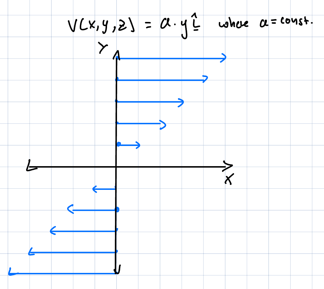
Example 2-D velocity field shown about the y-axis

Because the velocity depends on both position and time, fluid motion can become highly complex even for relatively simple geometries. This being said, for many flows, it is possible to neglect one or more coordinate components of the flow velocity, usually because the flow is considered to be uniform in that direction or because flow in that coordinate direction is not considered relevant to an engineering system.

In reality, all flows have a 3-D character, but 2-D flows, which describe flow kinematically in only two coordinate directions, and 1-D flows, which involves flow in only one coordinate direction, can be useful tools to simplify analyses. For instance, axisymmetric pipe flow, or flow between parallel plates is often considered in 2-D. Such simplifications always incur error; however, similar to solid mechanics, knowing when to simplify or reduce the order of a fluid system analysis can make solving a fluids problem more tractable.

Eulerian and Lagrangian Descriptions

Fluid motion may be described using either the Lagrangian or Eulerian perspective. In the Lagrangian description, individual fluid particles are tracked as they move through the flow field. The position, velocity, and acceleration of each particle are followed as functions of time. This approach is conceptually similar to tracking the trajectory of a single particle moving through space.

In contrast, the Eulerian description focuses on fixed points in space and examines how the flow properties vary at those locations. Instead of following individual particles, the velocity field is described everywhere within the domain at a given instant.

It is more common to see fluid flows analyzed from the Eulerian perspective; however, developing fluids principles in the Lagrangian formulation can occasionally be useful. Indeed, in other subjects like thermodynamics, where systems of particles with constant mass are studied, many core principles and formulae are developed in the Lagrangian of view.

Steady and Unsteady Flow

Flows are commonly classified according to whether one of its fluid properties (velocity, density etc.) changes with time at a specific point in space. Taking velocity as an example, a flow is considered steady if the velocity at every fixed point remains constant with time:

$$ \frac{\partial \vec{V}}{\partial t}=0 $$

For steady flow, the velocity at a particular location does not vary as time progresses. However, this does not necessarily mean that the velocity is uniform throughout the domain. Fluid particles may still accelerate if the velocity changes from one location to another.

If the velocity at a fixed point changes with time, the flow is classified as unsteady:

$$ \frac{\partial \vec{V}}{\partial t}\neq0 $$

As was demonstrated in Chapter 1 and 3 already, assuming steady flow frequently simplifies governing fluids equations by eliminating an independent variable in the flow domain - time. Strictly speaking, most flows have some degree of unsteadiness; however, many engineering systems are primarily concerned with operation at steady state conditions - after all transients have subsided - which can often be used to justify an assumption about steady flow conditions.

Flow Visualization

Several graphical descriptions are used to help visualize and interpret fluid motion.

Streamlines

A streamline is a curve that is tangent to the instantaneous velocity vector field at every point. This means that at any point along the streamline, the fluid velocity vector points directly along the curve. streamlines were already described and used extensively in Chapter 3.

For two-dimensional flow, the streamline equation is

$$ \frac{dy}{dx}=\frac{v}{u} $$

where $u$ and $v$ are the velocity components in the $x$- and $y$-directions.

Streamlines provide an instantaneous picture of the flow pattern and are especially useful for identifying specific behaviors. Among these streamlines can help identify flow separation around an object or reveal stagnation points.

Pathlines

A pathline represents the actual trajectory followed by an individual fluid particle as it moves through the flow field over time. Pathlines are obtained by tracking the motion of a specific particle.

Streaklines

A streakline is formed by all particles that previously passed through a particular point in the flow. It is common to see streaklines in flow visualization setups where a dye is used to color flow at particular point and track its motion thereafter through space and time.

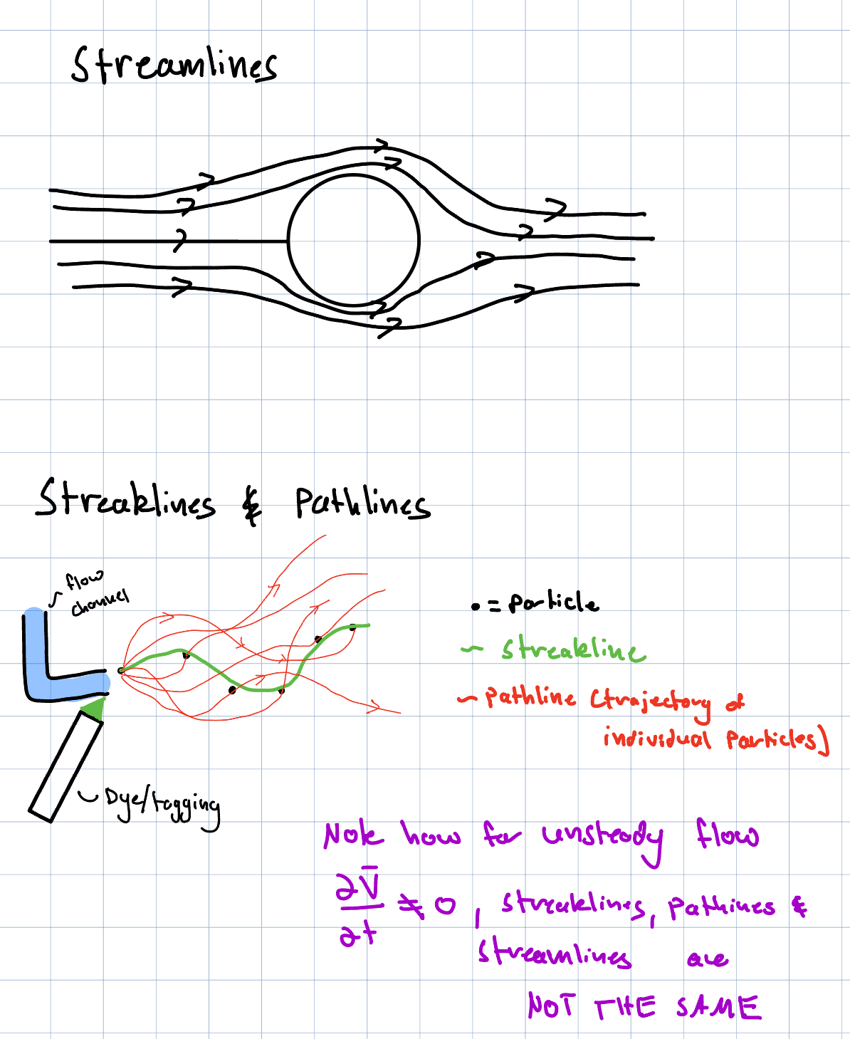
Overview of Streamlines, Streaklines, and Pathlines

Relationship Between the Different Lines

In steady flow, streamlines, pathlines, and streaklines are identical because the velocity field does not change with time.

In unsteady flow, these lines may differ substantially since the velocity field evolves as fluid particles move through the domain.

Acceleration Fields

While a velocity field describes how fast a fluid is moving, the acceleration field describes how the velocity changes throughout the flow. Fluid acceleration is important because it is directly related to the forces acting on the fluid through Newton's Second Law.

For a general velocity field,

$$ \vec{V}(x,y,z,t) = u\,\hat{i} + v\,\hat{j} + w\,\hat{k} $$

fluid particles may accelerate due to changes in time, changes in position, or both. As a result, acceleration can exist even in steady flow if the velocity varies spatially.

Material Derivative

In fluid mechanics, the acceleration of a fluid particle is determined using the material derivative. The material derivative represents the rate of change experienced by a moving fluid particle as it travels through the flow field.

The notation

$$ \frac{D}{Dt} $$

denotes the material derivative, where the capital $D$ indicates that the derivative follows the motion of a fluid particle rather than remaining at a fixed point in space. For any flow property $\phi$,

$$ \frac{D\phi}{Dt} = \frac{\partial \phi}{\partial t} + u\frac{\partial \phi}{\partial x} + v\frac{\partial \phi}{\partial y} + w\frac{\partial \phi}{\partial z} $$

The first term represents changes in $\phi$ in time at a fixed location, while the remaining terms account for changes experienced as the particle moves through regions with spatial variations.

When applied to the velocity field, the material derivative produces the fluid particle acceleration:

$$ \vec{a} = \frac{D\vec{V}}{Dt} $$

Local and Convective Acceleration

Expanding the material derivative gives

$$ \vec{a} = \frac{\partial \vec{V}}{\partial t} + u\frac{\partial \vec{V}}{\partial x} + v\frac{\partial \vec{V}}{\partial y} + w\frac{\partial \vec{V}}{\partial z} $$

The acceleration field therefore contains two distinct contributions. The term

$$ \frac{\partial \vec{V}}{\partial t} $$

is called the local acceleration. Again, this represents changes in velocity with time at a fixed point in space. A non-zero value for this partial derivative exists only in unsteady flow.

The remaining terms are called the convective acceleration. These terms arise because fluid particles move into regions where the velocity field changes spatially. Convective acceleration may exist even when the flow is steady. It is important to realize that even for steady flow, fluid properties, including velocity in a flow can change across space. However, at a fixed point in space, they will always be the same.

Acceleration Components

The acceleration components in Cartesian coordinates are

$$ a_x = \frac{Du}{Dt} = \frac{\partial u}{\partial t} + u\frac{\partial u}{\partial x} + v\frac{\partial u}{\partial y} + w\frac{\partial u}{\partial z} $$

$$ a_y = \frac{Dv}{Dt} = \frac{\partial v}{\partial t} + u\frac{\partial v}{\partial x} + v\frac{\partial v}{\partial y} + w\frac{\partial v}{\partial z} $$

$$ a_z = \frac{Dw}{Dt} = \frac{\partial w}{\partial t} + u\frac{\partial w}{\partial x} + v\frac{\partial w}{\partial y} + w\frac{\partial w}{\partial z} $$

These expressions form the basis for the momentum equations developed later in fluid mechanics.

Streamline Coordinates

As was discussed in Chapter 3, it is sometimes useful to discuss kinematic variables like acceleration in using the tangential-normal coordinate system, sometimes referred to as streamline coordinates. To reiterate this concept, the acceleration in the tangent or streamline $s$-direction and the normal $n$ direction can be written as

$$ \vec{a} = a_s\,\hat{e}_s + a_n\,\hat{e}_n $$

where:

$a_s$ is the tangential acceleration component
$a_n$ is the normal acceleration component

The tangential component is

$$ a_s = \frac{\partial V}{\partial t} + V\frac{\partial V}{\partial s} $$

which represents changes in the magnitude of the velocity.

The normal component is

$$ a_n = \frac{V^2}{R} $$

where again $R$ is the radius of curvature of the streamline.

Control Volume (CV) vs System Analysis

In fluid mechanics, problems can be approached in two different ways depending on how the fluid is being observed. The analysis may focus on a specific collection of fluid particles, called a system, or on a region in space through which fluid flows, called a control volume.

System Analysis

A system is a fixed amount of matter. The same fluid particles are tracked as they move through the flow field, meaning the system boundary moves and deforms with the fluid motion. Because the boundary always contains the same particles, no mass crosses the system boundary. This viewpoint is closely related to the Lagrangian description of fluid motion introduced earlier.

In principle, Newton's Laws are naturally written for systems. However, following individual fluid particles is often impractical because fluid regions continually change shape as the flow develops.

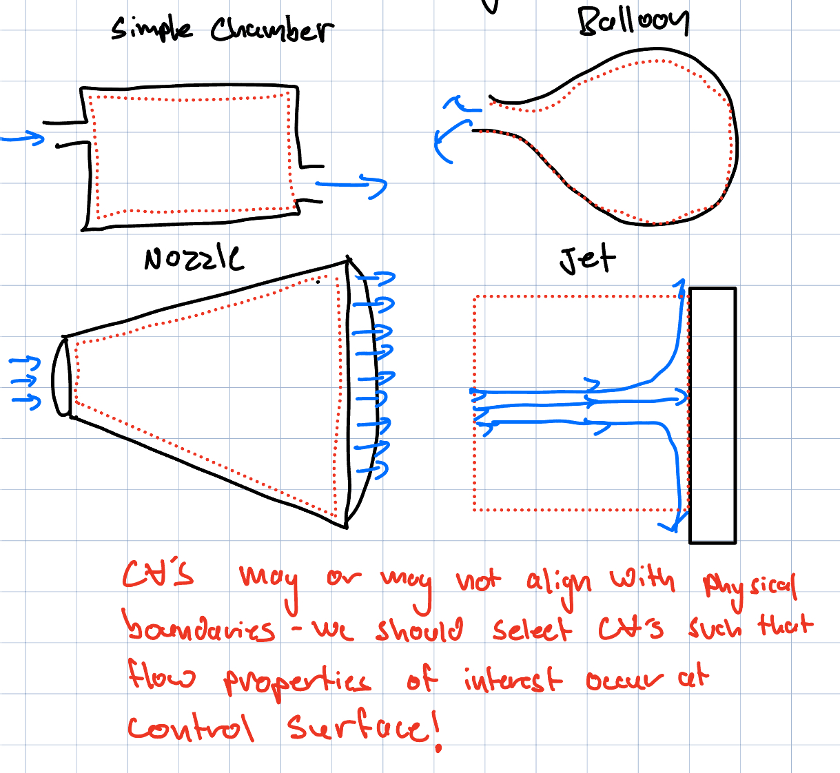
Control Volume Analysis

A control volume is a selected region in space used for analysis. Unlike a system, fluid is allowed to cross the control surface surrounding the region. It is in this way, a geometric object with which a flowing fluid interacts as opposed to a concrete selection of fluid particles. Control surfaces are what form the boundaries of the control volume.

Most engineering fluid mechanics problems are analyzed using control volumes because they simplify the study of flowing fluids in devices such as pipes, pumps, turbines, and nozzles.

Although a control volume does not track individual particles, it may still be:

fixed in space
moving
deforming with time

In many applications, a stationary control volume is used. As for the steady flow assumption, a fixed, stable control volume often simplifies a fluid mechanics problem, although it may not always be sufficient.

Consider a handful of simple control volumes to understand how they may be applied. Much like Free-Body Diagrams in mechanics, thoughtful selection of control volumes can simplify analyzes greatly.

Examples of Control Volumes

Importantly, the value of control volumes extends insofar as the first principles that have been developed for fluids principles can be applied. As a result, a control volume framework leads directly to the Reynolds Transport Theorem, which connects conservation laws written for systems to equivalent control volume formulations.

Reynolds Transport Theorem

The Reynolds Transport Theorem (RTT) provides the connection between the system viewpoint introduced earlier and the more practical control volume formulation used in most engineering fluid mechanics problems. Since the fundamental conservation laws are typically developed and written for system analysis, the RTT allows those laws to be rewritten in terms of a control volume through which fluid may flow.

In essence, the theorem states that the time rate of change of a property for a system can be expressed as the sum of:

the rate of change of that property within the control volume
the net rate at which the property crosses the control surface

This idea forms the basis for deriving the control volume forms of conservation of mass, momentum, and energy.

Extensive and Intensive Properties

The Reynolds Transport Theorem is written in terms of an extensive property, denoted by $B$. Extensive properties depend on the amount of matter present in the system. Common examples include:

mass
linear momentum
angular momentum
energy

Associated with every extensive property is an intensive property, defined as the amount of the extensive property per unit mass:

$$ b=\frac{B}{m} $$

This relationship allows system properties to be expressed locally throughout the flow field.

For example,

$$ b=1 \qquad \text{for mass} $$

$$ b=\vec{V} \qquad \text{for linear momentum} $$

$$ b=e \qquad \text{for energy} $$

where $e$ represents total energy per unit mass.

General Form of the Reynolds Transport Theorem

Using these definitions, the Reynolds Transport Theorem may be written as

$$ \frac{dB_{sys}}{dt} = \frac{\partial}{\partial t} \int_{CV} \rho b \, dV + \int_{CS} \rho b \, (\vec{V}\cdot\vec{n}) \, dA $$

where:

$ B_{sys} $ is the extensive property of the system
$ CV $ denotes the control volume
$ CS $ denotes the control surface
$ \rho $ is the fluid density
$ b $ is the corresponding intensive property
$ \vec{V} $ is the fluid velocity vector
$ \vec{n} $ is the outward unit normal vector to the control surface

The dot product

$$ \vec{V}\cdot\vec{n} $$

extracts the component of velocity normal to the control surface. This term is important because only velocity directed through the surface contributes to transport across the control volume boundary.

With the outward normal convention:

$ \vec{V}\cdot\vec{n} > 0 $ corresponds to flow leaving the control volume
$ \vec{V}\cdot\vec{n} < 0 $ corresponds to flow entering the control volume

The first term on the right-hand side,

$$ \frac{\partial}{\partial t} \int_{CV} \rho b \, dV $$

represents accumulation or depletion of the property within the control volume. The second term,

$$ \int_{CS} \rho b \, (\vec{V}\cdot\vec{n}) \, dA $$

represents the net transport of the property across the control surface due to fluid motion. Together, these terms account for all possible ways the system property can change.

Common Fluid Mechanics Applications

Once the general RTT expression is established, conservation equations can be developed simply by selecting the appropriate extensive property.

For conservation of mass,

$$ B=m \qquad \text{and} \qquad b=1 $$

which gives

$$ 0 = \frac{\partial}{\partial t} \int_{CV} \rho \, dV + \int_{CS} \rho (\vec{V}\cdot\vec{n}) \, dA $$

This is the integral form of the continuity equation.

For conservation of linear momentum,

$$ B=m\vec{V} \qquad \text{and} \qquad b=\vec{V} $$

which leads to

$$ \sum \vec{F} = \frac{\partial}{\partial t} \int_{CV} \rho \vec{V} \, dV + \int_{CS} \rho \vec{V}(\vec{V}\cdot\vec{n}) \, dA $$

This equation states that external forces acting on the control volume are balanced by momentum accumulation and momentum transport across the control surface. This is precisely a statement of Newton's 2nd Law, that the net force force acting on a system is the time rate of change of momentum of that system, only this time, the law has been formulated for a control volume approach. Conservation equations arrived at from RTT form the foundation for nearly all fluid mechanics analyses.

Moving and Deforming Control Volumes

The control volume itself does not need to remain stationary. In some applications, the control surface may move or deform with time, such as in rotating machinery, moving vehicles, piston-cylinder systems, or flexible boundaries.

A straightforward but common instance of this is when the control volume can be assumed to be moving at a constant velocity. When the control surface moves with velocity $ (\vec{n}_{CS}) $, the transport across the surface must be based on the velocity of the fluid relative to the moving boundary. The flux term therefore becomes

$$ (\vec{V}-\vec{V}_{CS})\cdot\vec{n} $$

and the RTT is modified to

$$ \frac{dB_{sys}}{dt} = \frac{\partial}{\partial t} \int_{CV} \rho b \, dV + \int_{CS} \rho b \, [(\vec{V}-\vec{V}_{CS})\cdot\vec{n}] \, dA $$

This form reduces to the standard stationary control volume equation when the control surface velocity is zero.

The Reynolds Transport Theorem is one of the most important tools in fluid mechanics because it provides a systematic way to convert conservation laws written for systems into practical equations that can be applied to real engineering devices and flowing fluids.