Particle kinematics

The two basic geometric objects we are using are positions and vectors. Positions describe locations in space, while vectors describe length and direction (no position information). To describe the kinematics (motion) of bodies we need to relate positions and vectors to each other.

Position vectors

Two positions P and Q can be used to define a vector $ \vec{r}_{PQ} = \vec{PQ} $ from P to Q. We call this the relative position of Q from P. If we start from the origin O, so we have $ \vec{r}_{OP} = \vec{OP} $, then we call this the position vector of position P. When it is clear, we will write $ \vec{r}_P $ for this position vector, or sometimes even just $ \vec{r} $.

Points $P$ and $Q$ and their relative and absolute position vectors. Note that we can write the position vectors with respect to different origins and in different bases.

Heads up!

Similar to particle kinematics, rigid body kinematics also builds on this content later in the course.

Rigid body kinematics examines the velocity and acceleration of particles on the same rigid body.

Transformation of position vectors

The position vector $ \vec{r}_{OP} $ a point P depends on which origin we are using. Using a different origin will result in a different position vector for the same point. The position vectors of a point from two different origins differ by the offset vector between the origins:

Change of origin for position vectors. #rkv-eo

$$ \begin{aligned} \overrightarrow{O_1 P} &= \overrightarrow{O_1 O_2} + \overrightarrow{O_2 P} \\ \vec{r}_{O_1 P} &= \vec{r}_{O_1 O_2} + \vec{r}_{O_2 P} \end{aligned} $$

Position vectors are defined by the origin and the point, but not by any choice of basis. We can write any position vector in any basis and it is still the same vector.

Basis for $ \vec{r}_{O_1P} $:

none $ \hat\imath,\hat\jmath $ $ \hat{u},\hat{v} $

Basis for $ \vec{r}_{O_1P} $:

none $ \hat\imath,\hat\jmath $ $ \hat{u},\hat{v} $

Velocity and acceleration vectors

The velocity $ \vec{v} $ and acceleration $ \vec{a} $ are the first and second derivatives of the position vector $ \vec{r} $. Technically, this is the velocity and acceleration relative to the given origin, as discussed in detail in the sections on relative motion and frames.

Definition of velocity and acceleration. #rkv-ev

$$ \begin{aligned} \vec{v} &= \dot{\vec{r}}\\ \vec{a} &= \dot{\vec{v}} \end{aligned} $$

The velocity can be decomposed into components parallel and perpendicular to the position vector, reflecting changes in the length and direction of $ \vec{r} $.

Decomposition of velocity and acceleration vectors. #rkv-ec

$$ \begin{aligned} \vec{v}_{proj} &= Proj(\vec{v}, \vec{r}) = \dot{r}\hat{r} \\ \vec{v}_{comp} &= Comp(\vec{v}, \vec{r}) = r\dot{\hat{r}} \\ \vec{a}_{proj} &= Proj(\vec{a}, \vec{v}) = \dot{v}\hat{v} \\ \vec{a}_{comp} &= Comp(\vec{a}, \vec{v}) = v\dot{\hat{v}} \end{aligned} $$

Velocity and acceleration of various movements. Compare to Figure #rvc-fp.

Application alert!

Track transition curves uses velocity and acceleration vectors.

Velocity and acceleration vectors can be used to analyze optimal road curves for driving.

Application alert!

Projectiles with air resistance uses velocity and acceleration vectors.

Velocity and acceleration vectors can be used to analyze objects following projectile motion with air resistance.

Velocity and acceleration in Cartesian basis

Differentiating in a fixed Cartesian basis can be done by differentiating each component.

Velocity and acceleration in cartesian basis. #rkv-er

$$ \begin{aligned} \vec{r} &= r_1 \hat\imath + r_2 \hat\jmath + r_3 \hat{k} \\ \vec{v} &= \dot{r}_1 \hat\imath + \dot{r}_2 \hat\jmath + \dot{r}_3 \hat{k} \\ \vec{a} &= \ddot{r}_1 \hat\imath + \ddot{r}_2 \hat\jmath + \ddot{r}_3 \hat{k} \end{aligned} $$

Summary table

	Cartesian	Polar
Position	$$ \vec{r} = x\hat\imath + y \hat\jmath $$	$$ \vec{r} = r \hat{e}_r $$
Velocity	$$ \vec{v} = \dot{x}\hat\imath + \dot{y} \hat\jmath $$	$$ \vec{v} = \dot{r} \hat{e}_r + r\dot{\theta}\hat{e}_\theta $$
Acceleration	$$ \vec{a} = \ddot{x}\hat\imath + \ddot{y} \hat\jmath $$	$$ \vec{a} = \frac{d}{dt} (\vec{v}) = \ddot{r} \hat{e}_r + \dot{\hat{e}_r} + \dot{r}\dot{\theta}\hat{e}_\theta\ + r\ddot{\theta}\hat{e}_\theta + r\dot{\theta}\dot{\hat{e}_\theta} $$ $$ \vec{a} = (\ddot{r} - r\dot{\theta}^2 ) \hat{e}_r + (2\dot{r}\dot{\theta} + r\ddot{\theta}) \hat{e}_\theta $$

Heads up!

Position velocity acceleration builds on this content in Mechanism design.

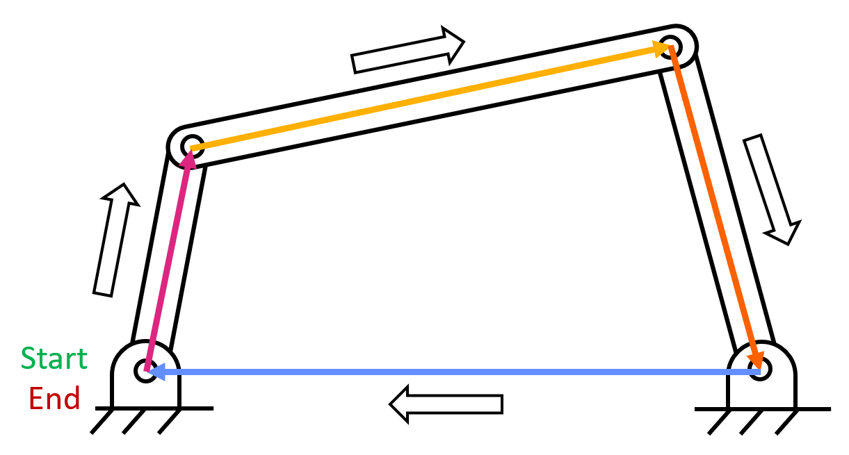
Position, Velocity, Acceleration (PVA) analysis is used to analytically determine the motion of a mechanism. Position determines the configuration of the mechanism, velocity determines the kinetic energy and momentum, and acceleration determines the forces. The known geometry, initial configurations, and PVA data of one link determines the PVA data for the other links.

Rotating frames

Angular velocity

A rotation of a vector is a change which only alters the direction, not the length, of a vector. A rotation consists of a rotation axis and a rotation rate. By taking the rotation axis as a direction and the rotation rate as a length, we can write the rotation as a vector, known as the angular velocity vector $ \vec{\omega} $. We use the right-hand rule to describe the direction of rotation. The units of $ \vec{\omega} $ are $\rm rad/s$ or $ {}^\circ/s $.

Rotation axis: $ \hat\imath $ $ \hat\jmath $ $ \hat{k} $ $ \hat\imath + \hat\jmath $ $ \hat\imath + \hat\jmath + \hat{k} $

Angular velocity vector $\vec\omega$. The direction of $\vec\omega$ is the axis of rotation, while the magnitude is the speed of rotation (positive direction given by the right-hand rule).

If an object is rotating with angular velocity $ \omega $ about a fixed origin, then the velocity and acceleration are given by the following relations:

Velocity and acceleration about a fixed origin. #rkv-ef

$$ \begin{aligned} \vec{v} &= \vec{\omega} \times \vec{r} \\ \vec{a} &= \vec{\alpha} \times \vec{r} + \vec{\omega} \times (\vec{\omega} \times \vec{r}) \end{aligned} $$

Did you know?

The Greek letter ω (lowercase omega) is the last letter of the Greek alphabet, leading to expressions such as “from alpha to omega” meaning “from start to end”. Omega literally means O-mega, meaning O-large, as capital Omega (written Ω) developed from capital Omicron (written Ο) by breaking the circle and turning up the edges. Omicron is literally O-micron, meaning O-small, and it is the ancestor of the Latin letter O that we use today in English.

Α	α	alpha	Ι	ι	iota	Ρ	ρ	rho
Β	β	beta	Κ	κ	kappa	Σ	σ	sigma
Γ	γ	gamma	Λ	λ	lambda	Τ	τ	tau
Δ	δ	delta	Μ	μ	mu	Υ	υ	upsilon
Ε	ε	epsilon	Ν	ν	nu	Φ	φ	phi
Ζ	ζ	zeta	Ξ	ξ	xi	Χ	χ	chi
Η	η	eta	Ο	ο	omicron	Ψ	ψ	psi
Θ	θ	theta	Π	π	pi	Ω	ω	omega

The Greek alphabet, shown above, was the first true alphabet, meaning that it has letters representing phonemes (basic significant sounds) and includes vowels as well as consonants. The Greek alphabet was was derived from the earlier Phoenician alphabet, which was probably the original parent of all alphabets. This shows that the idea of an alphabet is so non-obvious that it has only ever been invented once, and then always copied after that.

Application alert!

Celestial velocities uses angular velocity.

Angular velocity is an important variable to consider when analyzing celestial objects revolving around one another.

Vector derivatives and rotations

If a unit vector $ \hat{a} $ is rotating, then the angular velocity vector $ \vec{\omega} $ is defined so that:

Derivative of unit vectors. #rkr-ew

$$ \dot{\hat{a}} = \vec{\omega} \times \hat{a} $$

Derivative of general vectors. #rkr-ed

$$ \begin{aligned}\dot{\vec{a}} = \underbrace{\dot{a}\hat{a}}_{\operatorname{Proj}(\dot{\vec{a}}, \vec{a})} +\underbrace{\vec{\omega} \times\vec{a}}_{\operatorname{Comp}(\dot{\vec{a}}, \vec{a})}\end{aligned} $$

Using the same approach as #rvc-em we write $ \vec{a} =a\hat{a} $ and differentiate this and use rkr-ew to find:

$$ \begin{aligned}\dot{\vec{a}} &= \frac{d}{dt} \big( a \hat{a} \big) \\&= \dot{a} \hat{a} + a \dot{\hat{a}} \\&= \dot{a} \hat{a} + a (\vec\omega \times \hat{a}) \\&= \dot{a} \hat{a} + \vec\omega \times (a \hat{a}) \\&= \dot{a} \hat{a} + \vec\omega \times \vec{a}.\end{aligned} $$

Comparing this to #rvc-em shows that the two components are the projection and the complementary projection, respectively.

Derivative of constant-length vectors. #rkr-el

$$ \dot{\vec{a}} = \vec{\omega} \times \vec{a}\qquad\text{if $\vec{a}$ is constant length}\ $$

This can be seen from the fact that $ \dot{a} = 0 $ if $a$ is constant (a fixed length vector), substituted into #rkr-ed.

Rotations in 2D

In 2D the angular velocity can be thought of as a scalar (positive for counter-clockwise, negative for clockwise). This scalar is just the out-of-plane component of the full angular velocity vector. We can draw the angular velocity as either a vector pointing out of the plane, or as a circle-arrow in the plane, which is simpler for 2D diagrams.

Show:

Comparison of the vector and scalar representations of $\vec\omega$ for 2D rotations.

In 2D the angular velocity scalar $\omega$ is simply the derivative of the rotation angle $\theta$ in the plane:

Magnitude $\omega$ is derivative of angle $\theta$ in 2D. #rkr-e2

$$ \omega = \dot\theta $$

Take $ \hat{a} $ to be a unit vector rotating in the 2D $ \hat\imath–\hat\jmath $ plane, making an angle of $\theta$ with the $x$-axis, as in Figure #rkr-f2. Then:

$$ \hat{a} = \cos\theta \,\hat\imath + \sin\theta \,\hat\jmath. $$

Differentiating this expression gives:

$$ \dot{\hat{a}} = -\sin\theta \, \dot\theta \,\hat\imath+ \cos\theta \,\dot\theta \,\hat\jmath. $$

We now consider an angular velocity vector $\vec\omega$. Because the rotation is in the $\hat\imath$–$\hat\jmath$ plane, the angular velocity vector must be in the $ \hat{k} $ direction. Thus $ \vec\omega = \omega \hat{k} $. Now we can compute the derivative of $ \hat{a} $ using #rkr-ew, giving:

$$ \begin{aligned}\dot{\hat{a}} &= \vec\omega \times \hat{a} \\&= \omega\hat{k} \times \big( \cos\theta \,\hat\imath+ \sin\theta \,\hat\jmath \big) \\&= \omega \cos\theta \,(\hat{k} \times \hat\imath)+ \omega \sin\theta \,(\hat{k} \times \hat\jmath) \\&= \omega \cos\theta \,\hat\jmath+ \omega \sin\theta \,(-\hat\imath) \\&= - \omega \sin\theta \,\hat\imath+ \omega \cos\theta \,\hat\jmath.\end{aligned} $$

Comparing this expression to the earlier one for $ \dot{\hat{a}} $we see that $\omega = \dot\theta$.

The right-hand rule convention for angular velocities means that counter-clockwise rotations are positive, just like the usual angle direction convention.

Did you know?

Angular directions have long been considered to have magical or spiritual significance. In Britain the counterclockwise direction was once known as widdershins, and it was considered unlucky to travel around a church in a widdershins direction.

Interestingly, right-handed people tend to naturally draw circles in a counterclockwise direction, and clockwise drawing in right-handed children is an early warning sign for the later development of schizophrenia [Blau, 1977].

References

T. H. Blau. Torque and schizophrenic vulnerability. American Psychologist, 32(12):997–1005, 1977. DOI: 10.1037/0003-066X.32.12.997.

Rotations and vector “positions”

The fact that vectors don't have positions means that vector rotations are independent of where vectors are drawn, just like for derivatives.

Show:

Rotational motion of vectors which are drawn moving about. Note that the drawn position does not affect the angular velocity $\omega$ or the derivative vectors.

Properties of rotations

Rotations are rigid transformations, meaning that they keep constant all vector lengths and all relative vector angles. These facts are reflected in the following results, which all consider two vectors $ \vec{a} $ and $ \vec{b} $ that are rotating with angular velocity $ \vec\omega $.

Derivative of rotating vector is orthogonal. #rkr-e2a

$$ \dot{\vec{a}} \cdot \vec{a} = 0 $$

Using #rkr-el and the scalar triple product formula #rvi-es gives:

$$ \begin{aligned}\vec{a} \cdot \dot{\vec{a}}&= \vec{a} \cdot \big( \vec{\omega} \times \vec{a} \big) \\&= \vec{\omega} \cdot \big( \vec{a} \times \vec{a} \big) \\&= 0.\end{aligned} $$

Angle $\theta$ between rotating vectors is constant. #rkr-e2b

$$ \theta = \cos^{-1}\left(\frac{\vec{b} \cdot\vec{a}}{b a}\right) = \text{constant} $$

We first consider the dot product $ \vec{a} \cdot \vec{b} $ and show that this is not changing with time. We do this by using the scalar triple product formula #rvi-es to find:

$$ \begin{aligned}\frac{d}{dt} \big( \vec{a} \cdot \vec{b} \big)&= \dot{\vec{a}} \cdot \vec{b} + \vec{a} \cdot \dot{\vec{b}} \\&= (\vec{\omega} \times \vec{a}) \cdot \vec{b} + \vec{a} \cdot (\vec{\omega} \times \vec{b}) \\&= \vec{b} \cdot (\vec{\omega} \times \vec{a}) + \vec{b} \cdot (\vec{a} \times \vec{\omega}) \\&= \vec{b} \cdot (\vec{\omega} \times \vec{a}) - \vec{b} \cdot (\vec{\omega} \times \vec{a}) \\&= 0.\end{aligned} $$

Now $ \vec{a} \cdot \vec{b} $ is constant and the lengths $a$ and $b$ are constant, so the angle $\theta$ between the vectors must be constant.

Rotating vectors parallel to $\vec\omega$ are constant. #rkr-e2c

$$ \dot{\vec{a}} = 0 \qquad \text{if $\vec{a}$ is rotating and parallel to $\vec\omega$} $$

From #rkr-el we know that the derivative is

$$ \dot{\vec{a}} = \vec\omega \times \vec{a}, $$

but the cross product is zero for parallel vectors, so this the derivative is zero.

Rodrigues’ rotation formula

Rodrigues’ rotation formula gives an explicit formula for a vector rotated by an angle about a given axis.

Rodrigues’ rotation formula for $\vec{a}$ rotated by $\theta$ about $\hat{b}$. #rkr-er

$$ \operatorname{Rot}(\vec{a}; \theta, \hat{b}) =\vec{a} \cos\theta + (\hat{b} \times\vec{a}) \sin\theta + \hat{b} (\hat{b} \cdot\vec{a}) (1 - \cos\theta) $$

Assume $ \vec{a} $ is not parallel to $ \hat{b} $. Then let $ \vec{v} = \hat{b} \times \vec{a} $ and $ \vec{u} = \vec{v} \times \vec{b} $, so $ \hat{u}, \hat{v}, \hat{b} $ is a right-handed orthonormal basis. Take $\phi$ to be the angle between $ \vec{a} $ and $ \hat{b} $. Then we do a rotation by $\theta$ in the $ \hat{u}-\hat{v} $ plane:

$$ \begin{aligned} \vec{a} &= a \sin\phi\,\hat{u} + a \cos\phi \,\hat{b} \\\operatorname{Rot}(\vec{a};\theta,\hat{b}) &= a\cos\theta \sin\phi \,\hat{u} + a \sin\theta \sin\phi\,\hat{v} + a \cos\phi \,\hat{b}.\end{aligned} $$

Now we want to convert from the $ \hat{u},\hat{v},\hat{b} $ basis to write the rotated result in terms of $ \vec{a}, \hat{b} \times \vec{a}), \hat{b} $. To do this, we need to work out what $ \hat{u},\hat{v},\hat{b} $are in terms of these other vectors.

$$ \begin{aligned} \hat{v} &= \frac{\hat{b} \times\vec{a}}{\|\hat{b} \times \vec{a}\|} =\frac{\hat{b} \times \vec{a}}{a \sin\phi} \\\hat{u} &= \frac{\vec{v} \times\hat{b}}{\|\vec{v} \times \vec{b}\|} =\frac{\vec{v} \times \hat{b}}{a \sin\phi} =\frac{(\hat{b} \times \vec{a}) \times \hat{b}}{a\sin\phi} = \frac{\hat{b} \times (\vec{a} \times\hat{b})}{a \sin\phi} \\&= \frac{\vec{a} - (\hat{b}\cdot \vec{a}) \hat{b}}{a \sin\phi} = \frac{1}{a\sin\phi} \vec{a} - \frac{\hat{b} \cdot\vec{a}}{a \sin\phi} \hat{b}.\end{aligned} $$

Substituting these into the rotated vector expression above gives

$$ \begin{aligned}\operatorname{Rot}(\vec{a};\theta,\hat{b}) &= a\cos\theta \sin\phi \, \left( \frac{1}{a \sin\phi}\vec{a} - \frac{\hat{b} \cdot \vec{a}}{a\sin\phi} \hat{b} \right) \\& \qquad + a \sin\theta \sin\phi \, \left(\frac{\hat{b} \times \vec{a}}{a \sin\phi} \right)+ a \cos\phi \,\hat{b} \\ &= \cos\theta\,\vec{a} - \cos\theta \,(\hat{b} \cdot\vec{a}) \,\hat{b} + \sin\theta \,(\hat{b} \times\vec{a}) + a\cos\theta \,\hat{b} \\ &=\cos\theta \,\vec{a} + (1 - \cos\theta) (\hat{b}\cdot \vec{a}) \,\hat{b} + \sin\theta \,(\hat{b}\times \vec{a}).\end{aligned} $$

Angular acceleration

In polar coordinates, acceleration consists of both radial and tangential components. The tangential component is directly related to changes in the angular velocity, which introduces the concept of angular acceleration.

Angular acceleration, denoted as $ \ddot{\theta} $ represents the rate of change of angular velocity $ \dot{\theta} $ with respect to time. It appears as part of the total acceleration in the tangential direction, described by the unit vector $ \hat{e}_{\theta} $. The full expression for the acceleration in polar coordinates is:

$$ \vec{a} = (\ddot{r} - r\dot{\theta}^2) \hat{e}_r + (r\ddot{\theta} + 2\dot{r}\dot{\theta}) \hat{e}_\theta $$

Here, the first term of the equation represents the radial component, described by the unit $ \hat{e}_r $, and the second term is the angular component, described by the vector unit $ \hat{e}_{\theta} $. In the radial component, there is a radial ($ \ddot{r} $) and a centripetal ($ r\dot{\theta}^2 $) term. In the angular component, there is an angular ($ r\ddot{\theta} $) and a coriolis ($ 2\dot{r}\dot{\theta} $) term.

Tangential and normal basis

Normal basis

Consider a particle moving with position vector $ \vec{r} $ and corresponding velocity $ \vec{v} $ and acceleration $ \vec{a} $. The tangential/normal basis $ \hat{e}_t,\hat{e}_n,\hat{e}_b $ is:

Tangential/normal basis vectors. #rkt-eb

$$ \begin{aligned}\hat{e}_t &= \hat{v}& &\text{tangential basis vector} \\\hat{e}_n &= \frac{\dot{\hat{e}}_t}{\|\dot{\hat{e}}_t\|}= \frac{\operatorname{Comp}(\vec{a},\vec{v})}{\|\operatorname{Comp}(\vec{a},\vec{v})\|}& &\text{normal basis vector} \\\hat{e}_b &= \hat{e}_t \times \hat{e}_n& &\text{binormal basis vector} \\\end{aligned} $$

These equations are definitions of the basis vectors, so the only thing to derive is the alternative formula for $ \hat{e}_n $. Using the definition of $ \hat{e}_t $ above and #rvc-eu, we see that

$$ \dot{\hat{e}}_t = \dot{\hat{v}} = \frac{1}{v} \operatorname{Comp}(\dot{\vec{v}}, \vec{v}) = \frac{1}{v} \operatorname{Comp}(\vec{a}, \vec{v}). $$

Normalizing both sides gives the desired expression:

$$ \frac{\dot{\hat{e}}_t}{\|\dot{\hat{e}}_t\|} = \frac{\frac{1}{v} \operatorname{Comp}(\vec{a}, \vec{v})}{ \left\|\frac{1}{v} \operatorname{Comp}(\vec{a}, \vec{v})\right\|} = \frac{\frac{1}{v} \operatorname{Comp}(\vec{a}, \vec{v})}{ \frac{1}{v} \|\operatorname{Comp}(\vec{a}, \vec{v})\|} = \frac{\operatorname{Comp}(\vec{a}, \vec{v})}{ \|\operatorname{Comp}(\vec{a}, \vec{v})\|}. $$

The tangential basis vector $ \hat{e}_t $ points tangential to the path, the normal basis vector $ \hat{e}_n $ points perpendicular (normal) to the path towards the instantaneous center of curvature, and the binormal basis vector $ \hat{e}_b $ completes the right-handed basis.

Show:

Tangential/normal basis associated with movement around a curve in 3D. Observe that the velocity $ \vec{v} $ is always in the $ \hat{e}_t $ direction and that the acceleration $ \vec{a} $ always lies in the $ \hat{e}_t,\hat{e}_n $ plane (the osculating plane). The center of curvature and osculating circle are defined below.

Curvature and torsion

Curvature and torsion. #rkt-ek

To better understand the geometry of the tangential/normal basis, we can use the curvature $\kappa$ to describe the curving of the path, and the torsion $\tau$ to describe the rotation of the basis about the path. These quantities are defined by:

$$ \begin{aligned}\kappa &= \frac{d\hat{e}_t}{ds} \cdot \hat{e}_n= \frac{1}{v} \dot{\hat{e}}_t \cdot \hat{e}_n & &\text{curvature} \\\rho &= \frac{1}{\kappa} & &\text{radius of curvature} \\\tau &= -\frac{d\hat{e}_b}{ds} \cdot \hat{e}_n= -\frac{1}{v} \dot{\hat{e}}_b \cdot \hat{e}_n & &\text{torsion} \\\sigma &= \frac{1}{\tau} & &\text{radius of torsion}\end{aligned} $$

These equations are definitions, so we need only check that the two expressions for each of $\kappa$ and $\tau$ are equivalent. This follows immediately, however, from the chain-rule conversions #rkt-ea between $d/ds$ and $d/dt$.

The radius of curvature $\rho$ is the radius of equivalent circular motion, and the torsion determines the rate of rotation of the osculating plane, as described below in a section below.

Basis derivatives and angular velocity

As the point $P$ moves along its path, the associated tangential/normal basis rotates with an angular velocity vector $\omega$ given by:

Angular velocity of the tangential/normal basis. #rkt-ew

$$ \begin{aligned}\vec{\omega} &= v\tau \,\hat{e}_t + v \kappa \,\hat{e}_b\end{aligned} $$

We start by writing the angular velocity in the tangential/normal basis, giving:

$$ \vec{\omega} = \omega_t\,\hat{e}_t + \omega_n\,\hat{e}_n+ \omega_b\,\hat{e}_b. $$

Now the basis vector derivatives are given by the cross product by $ \vec{\omega} $ from #rkr-ew, so we can evaluate the expressions #rkt-ek for curvature and torsion to give:

$$ \begin{aligned}\kappa &= \frac{1}{v} \dot{\hat{e}}_t \cdot \hat{e}_n \\&= \frac{1}{v} (\vec{\omega} \times \hat{e}_t) \cdot \hat{e}_n \\&= \frac{1}{v} (\omega_b\,\hat{e}_n - \omega_n\,\hat{e}_b) \cdot \hat{e}_n \\&= \frac{1}{v} \omega_b\end{aligned} $$

and

$$ \begin{aligned}\tau &= -\frac{1}{v} \dot{\hat{e}}_b \cdot \hat{e}_n \\&= -\frac{1}{v} (\vec{\omega} \times \hat{e}_b) \cdot \hat{e}_n \\&= -\frac{1}{v} (\omega_n\,\hat{e}_t - \omega_t\,\hat{e}_n) \cdot \hat{e}_n \\&= \frac{1}{v} \omega_t.\end{aligned} $$

Rearranging the final expressions in each case gives $ \omega_b = v\kappa $ and $ \omega_t = v\tau $. From the definition #rkt-eb of $ \hat{e}_n $, we see that

$$ \begin{aligned}\hat{e}_n &= \frac{\dot{\hat{e}}_t}{\|\dot{\hat{e}}_t\|} \\\hat{e}_n \cdot \hat{e}_b &= \frac{1}{\|\dot{\hat{e}}_t\|} (\vec{\omega} \times \hat{e}_t) \cdot \hat{e}_b \\0 &= \frac{1}{\|\dot{\hat{e}}_t\|} (\omega_b\,\hat{e}_n - \omega_n\,\hat{e}_b) \cdot \hat{e}_b \\&= - \frac{1}{\|\dot{\hat{e}}_t\|} \omega_n.\end{aligned} $$

from which we conclude that $ \omega_n = 0 $, giving us all three components of $ \vec{\omega} $.

Knowing the angular velocity vector of the tangential/normal basis allows us to easily compute the time derivatives of each tangential/normal basis vector, as follows:

Tangential/normal basis vector derivatives. #rkt-ed

$$ \begin{aligned}\dot{\hat{e}}_t &= \phantom{-v\kappa\,\hat{e}_t - } v\kappa\,\hat{e}_n \\\dot{\hat{e}}_n &= -v\kappa\,\hat{e}_t \phantom{ - v\kappa\,\hat{e}_n + } + v\tau\,\hat{e}_b \\\dot{\hat{e}}_b &=\phantom{-v\kappa\,\hat{e}_t } - v\tau\,\hat{e}_n\end{aligned} $$

We can use the expression #rkt-ew for $ \vec{\omega} $ together with #rkr-ew to find the basis vector derivatives:

$$ \begin{aligned}\dot{\hat{e}}_t &= \vec{\omega} \times \hat{e}_t= (v\tau \,\hat{e}_t + v \kappa \,\hat{e}_b) \times \hat{e}_t= v \kappa \,\hat{e}_n \\\dot{\hat{e}}_n &= \vec{\omega} \times \hat{e}_n= (v\tau \,\hat{e}_t + v \kappa \,\hat{e}_b) \times \hat{e}_n= - v \kappa \,\hat{e}_t + v \tau \,\hat{e}_b \\\dot{\hat{e}}_b &= \vec{\omega} \times \hat{e}_b= (v\tau \,\hat{e}_t + v \kappa \,\hat{e}_b) \times \hat{e}_b= -v \tau \,\hat{e}_n.\end{aligned} $$

Notation note

The tangential/normal basis is also called the Frenet–Serret frame after Jean Frédéric Frenet and Joseph Alfred Serret, who discovered it independently around 1850. The equations #rkt-ed for the basis derivatives are often called the Frenet-Serret formulas, typically written in terms of $s$ derivatives:

$$ \begin{aligned}\frac{d\hat{e}_t}{ds} &= \phantom{-\kappa\,\hat{e}_t - } \kappa\,\hat{e}_n \\\frac{d\hat{e}_n}{ds} &= -\kappa\,\hat{e}_t \phantom{ - \kappa\,\hat{e}_n + } + \tau\,\hat{e}_b \\\frac{d\hat{e}_b}{ds} &=\phantom{-\kappa\,\hat{e}_t } - \tau\,\hat{e}_n.\end{aligned} $$

If we divide the angular velocity vector #rkt-ew by $v$ then we obtain the vector

$$ \frac{1}{v} \vec{\omega} = \tau\,\hat{e}_t + \kappa\,\hat{e}_b, $$

which is known as the Darboux vector after its discoverer, Jean Gaston Darboux.

Tangent lines and osculating circles

Given a point $P$ moving along a complex path, at a given instant of time we can match different components of the point's motion with successively more complex geometric shapes:

match	geometric object	name
$ \vec{r} $	point	position
$ \vec{r},\vec{v} $	line	tangent line
$ \vec{r},\vec{v},\vec{a} $	circle	osculating circle

The osculating circle is the instantaneous equivalent circular path. That is, a particle traveling on the osculating circle with the same location $P$, speed $ \dot{s} $, and tangential acceleration $ \ddot{s} $ as our particle would have matching velocity and acceleration vectors.

Osculating circle #rkt-eo

$$ \text{center C} = \vec{r} + \rho \hat{e}_n,\qquad \text{radius} \; \rho,\qquad \text{normal to} \; \hat{e}_b $$

Consider a particle $P$ with position vector $ \vec{r}_P $ moving with velocity $ \vec{v}_P $ and acceleration $ \vec{a}_P $ , and let $ \hat{e}_t,\hat{e}_n,\hat{e}_b $be the associated tangential/normal basis and $ \rho_P $ be the radius of curvature. Set $ \dot{s}_P = v_P $and $ \ddot{s}_P = \vec{a}_P \cdot \hat{e}_t $ to be the speed and tangential acceleration of $P$.

Next define the osculating circle as above with center $ C = \vec{r}_P + \rho_P $ , radius $ \rho_P $, and normal vector $ \hat{e}_b $.

Now take a second particle $Q$ moving on the osculating circle so that its instantaneous position matches $P$ and it has the same speed $ \dot{s}_Q = \dot{s}_P $ and tangential acceleration $ \ddot{s}_Q = \ddot{s}_P $. This means that the radius of the circle $ r_Q $ for $Q$ is matches the osculating circle radius $ \rho_P $, so $ r_Q = \rho_P $.

We want to prove that $ \vec{v}_Q = \vec{v}_P $ and $ \vec{a}_Q = \vec{a}_P $.

We will use a polar coordinate system for $Q$, centered at $C$ and in the plane with normal vector $ \hat{e}_b $. At the current instant when the particles are at the same position, this means that $ \hat{e}_r = -\hat{e}_n $ and $ \hat{e}_\theta = \hat{e}_t $. Using the circular motion expressions #rke-ec we have that the velocity of $Q$ is:

$$ \begin{aligned} \vec{v}_Q &= v_Q \,\hat{e}_\theta \\ &= \dot{s}_Q \,\hat{e}_\theta \\ &= \dot{s}_P \,\hat{e}_t = \vec{v}_P. \\ \end{aligned} $$

For a particle moving in a circle like $Q$, the speed is given by $ \dot{s}_Q = v_Q = r_Q \omega_Q $, and differentiating this gives $ \ddot{s}_Q = r_Q \dot{\omega}_Q = r_Q \alpha_Q $. Using this, the acceleration of $Q$ is:

$$ \begin{aligned} \vec{a}_Q &= -\frac{v_Q^2}{\rho_Q} \,\hat{e}_r + \rho_Q \alpha_Q \,\hat{e}_\theta \\ &= -\frac{\dot{s}_Q^2}{\rho_Q} \,\hat{e}_r + \ddot{s}_Q \,\hat{e}_\theta \\ &= \frac{\dot{s}_P^2}{\rho_P} \,\hat{e}_n + \ddot{s}_Q \,\hat{e}_t \\ &= \vec{a}_Q. \end{aligned} $$

We thus see that points $P$ and $Q$ have the same instantaneous velocity and acceleration. This also means that the tangential/normal basis computed at this instant for $Q$ will match that of $P$.

The osculating circle lies in the $ \hat{e}_t,\hat{e}_n $ plane, which is thus called the osculating plane. This plane has normal vector $ \hat{e}_b $, and rotates about $ \hat{e}_t $ with a rotation rate determined by the torsion $\tau$, as we see from the expression #rkt-ed for the derivative of $ \hat{e}_b. $

Show:

Match phase: 0%

Tangent lines and osculating circles, showing matching of velocity or velocity and acceleration, respectively.

Curvature on curves

Given a parametric curve, its curvature can be directly evaluated with:

Curvature of parametric curve $\vec{r}(u)$ in 3D. #rkt-ec

$$ \kappa = \frac{\|\vec{r}' \times \vec{r}''\|}{\|\vec{r}'\|^3} $$

Because the tangential/normal basis vectors #rkt-eb are all normalized, it does not matter how fast the point moves along the line. We can thus evaluate the parametric curve as a function of time, giving $ \vec{r}(t) $. Now:

$$ \begin{aligned}\|\vec{r}'' \times \vec{r}'\| &= \|\vec{a} \times \vec{v}\| \\&= a v \sin\theta \\&= \frac{v^3}{\rho},\end{aligned} $$

where we used the cross product length formula #rvv-el and equation #rkt-er for the radius of curvature $ \rho $. By definition #rkt-ek the curvature is $ \kappa = 1/\rho $, so

$$ \begin{aligned}\|\vec{r}'' \times \vec{r}'\|&= v^3 \kappa \\\kappa &= \frac{\|\vec{r}'' \times \vec{r}'\|}{\|\vec{r}'\|^3}.\end{aligned} $$

While the above formula can be used in 2D by taking the third component to be zero, it can also be written in an explicitly 2D form:

Curvature of parametric curve $x = x(u)$, $y = y(u)$ in 2D. #rkt-e2

$$ \kappa = \frac{|x''y' - y''x'|}{(x'^2 + y'^2)^{3/2}} $$

This equation is just #rkt-ec written in explicit 2D coordinates. To see this, we first take the position vector $ \vec{r}(u) $ to be

$$ \vec{r}(u) = x(u)\,\hat\imath + y(u)\,\hat\jmath. $$

Now $ r'(u) = \sqrt{(x'(u))^2 + (y'(u))^2} $ and

$$ \begin{aligned}\vec{r}'' \times \vec{r}'&= (x''\,\hat\imath + y''\,\hat\jmath)\times (x'\,\hat\imath + y'\,\hat\jmath) \\&= (x''y' - y''x')\,\hat{k},\end{aligned} $$

so evaluating #rkt-ec gives the desired expression.

We can take this a step further, and obtain an expression for an explicitly defined function.

Curvature of an explicitly defined function $y = f(x).$ #rkt-e3

$$ \kappa = \frac{|y''(x)|}{(1 + y'(x)^2)^{3/2}} $$

Use equation #rkt‑e2 and parametrize the curve using $x$ as the parametrization variable. Namely:

$$ \begin{aligned}x = u, \quad \quad y = y(u) = y(x)\end{aligned} $$

This yields a very elegant expression, as $ x'(u) = 1 $ and $ x''(u) = 0 $, which lets us arrive at the desired expression #rkt‑e3.

System comparison: Cartesian/polar/tangent-normal

	Cartesian	Polar	Tangent-Normal
Position	$$ \vec{r} = x\hat\imath + y \hat\jmath $$	$$ \vec{r} = r \hat{e}_r $$	$$ s $$
Velocity	$$ \vec{v} = \dot{x}\hat\imath + \dot{y} \hat\jmath $$	$$ \vec{v} = \dot{r} \hat{e}_r + r\dot{\theta}\hat{e}_\theta $$	$$ \vec{v} = \dot{s}\hat{e}_t $$
Acceleration	$$ \vec{a} = \ddot{x}\hat\imath + \ddot{y} \hat\jmath $$	$$ \vec{a} = (\ddot{r} - r\dot{\theta}^2 ) \hat{e}_r + (2\dot{r}\dot{\theta} + r\ddot{\theta}) \hat{e}_\theta $$	$$ \vec{a} = \ddot{s}\hat{e}_t + \dot{s}^2 \kappa \hat{e}_n $$

Show:
Movement:	circle	var-circle	ellipse	arc
	trefoil	eight	comet	pendulum
Show:

Movement:	circle	var-circle	ellipse	arc
	trefoil	eight	comet	pendulum
Show:

Origin:	\(O_1\)	\(O_2\)

Movement:	circle	var-circle	ellipse	arc
	trefoil	eight	comet	pendulum
Show:

Origin:	\(O_1\)	\(O_2\)

Particle kinematics

Position vectors

Transformation of position vectors

Velocity and acceleration vectors

Velocity and acceleration in Cartesian basis

Velocity and acceleration in polar basis

Summary table

Rotating frames

Angular velocity

Vector derivatives and rotations

Rotations in 2D

References

Rotations and vector “positions”

Properties of rotations

Rodrigues’ rotation formula

Angular acceleration

Tangential and normal basis

Normal basis

Curvature and torsion

Basis derivatives and angular velocity

Normal and tangential kinematics

Tangent lines and osculating circles

Curvature on curves

System comparison: Cartesian/polar/tangent-normal

Learn More

match	geometric object	name
\( \vec{r} \)	point	position
\( \vec{r},\vec{v} \)	line	tangent line
\( \vec{r},\vec{v},\vec{a} \)	circle	osculating circle