Current page:

Power Cycles

Much of the power that we use in our daily lives is produced through cycles operating with a working fluid.

Carnot cycle

A Carnot cycle is defined as an ideal gas, undergoing a 4-step, reversible, closed thermodynamic cycle. Imagine that an ideal gas contained within a piston-cylinder undergoes the series of processes depicted in Fig. CarnotCycle below, with the gas starting in state $ 1 $ before progressing to states $ 2 $, $ 3 $, $ 4 $, and then returning to state $ 1 $ to complete a cycle.

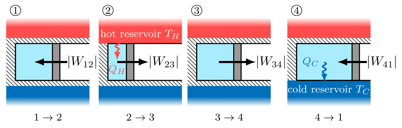
Figure 1: A schematic of a piston-cylinder executing a Carnot cycle between hot and cold thermal reservoirs.

During the cycle, the system contacts sequentially a hot reservoir and a cold reservoir at temperatures $ T_H $ and $ T_C $, respectively. While in contact with a thermal reservoir, the system remains at the temperature of the thermal reservoir. In between reservoir contacts, the system is insulated and no heat transfer occurs. Each process quasi-static, and reversible. In this idealized cycle, heat transfers in and out of the system despite the fact that there is no temperature difference to drive heat flow. Such hypothetical heat flow is reversible because an infinitesimal increase in the reservoir temperature relative to the system will cause heat to flow into the system, or vice versa for an infinitesimal decrease in the reservoir temperature. This idealized cycle is known as a Carnot cycle.

Reversible process:

In a reversible process, the direction can be reversed at any point by an infinitesimal change in external conditions.

Quasi-static process:

A process that occurs at an infinitesimally slow rate so that the system is in a thermodynamic equilibrium at all times.

Carnot Cycle Steps

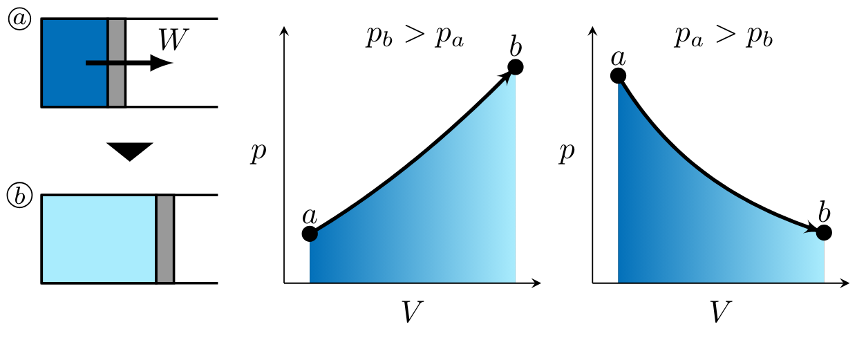
In processes $ 2 \to 3 $ and $ 3 \to 4 $, work is done by the gas. Figure PVwork1 illustrates two potential, monotonic processes corresponding to positive work, or work done by the gas. On the left, pressure is higher in state $ b $ than state $ a $. On the right, pressure is higher in state $ a $ than state $ b $. $ V_b > V_a $ in both cases. When illustrating the magnitude of the work to be determined, the arrow is drawn out of the system as shown in state $ 1 $.

Figure 2: Work done by the gas

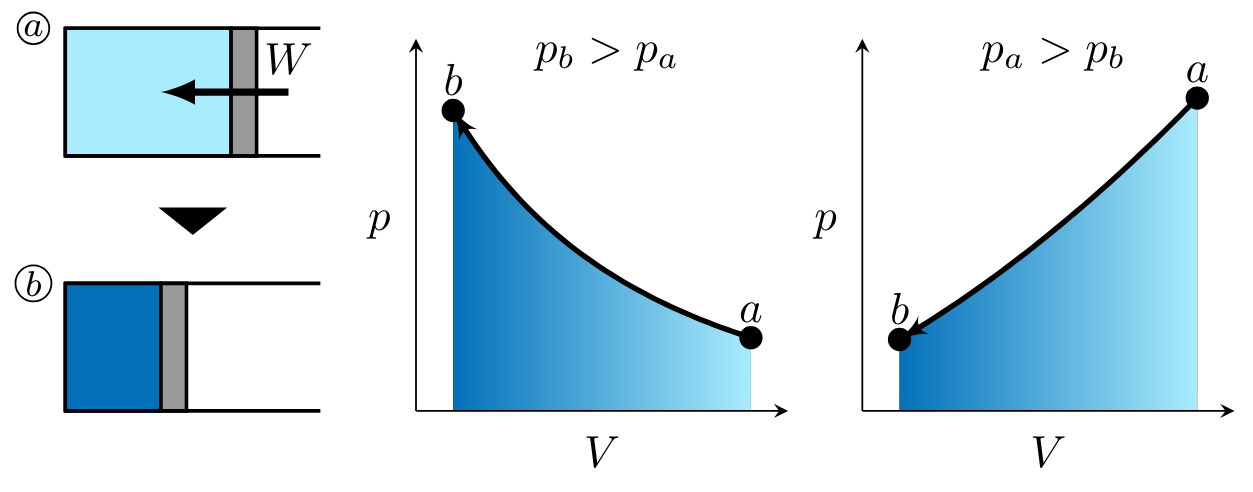
In processes $ 1 \to 2 $ and $ 4 \to 1 $, work is done on the gas. Figure PVwork1 illustrates two potential, monotonic processes corresponding to positive work, or work done by the gas. On the left, pressure is higher in state $ b $ than state $ a $. On the right, pressure is higher in state $ a $ than state $ b $. $ V_a > V_b $ in both cases as shown in Figure PVwork2. Recall the expression for $ pV $ work,

$$ W = \int_{V_a}^{V_b} p(V) dV, $$

noting that work for these processes is negative as indicated by the right-to-left process curve arrow in each of the $ pV $ diagrams. When illustrating the magnitude of the work to be determined, the arrow is drawn into the system as shown in state $ a $ (Fig. PVwork2).

Figure 3: Work done on the gas

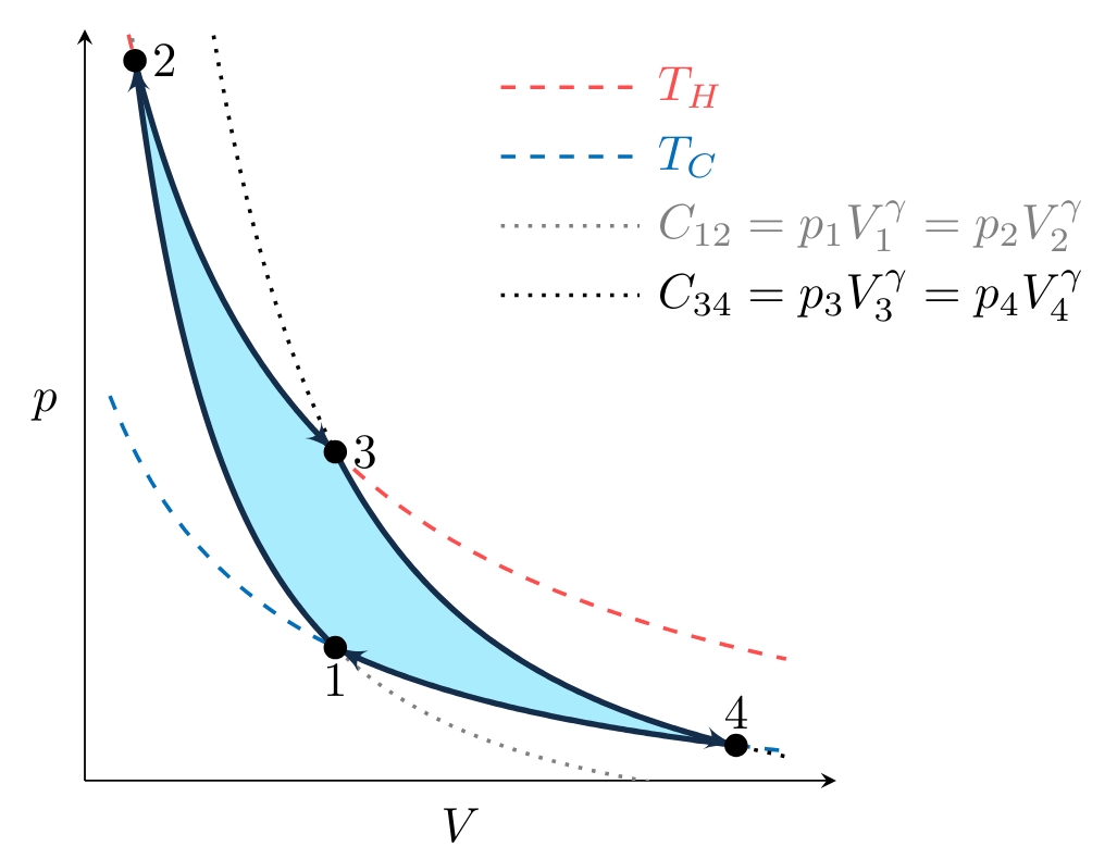
To plot the processes that make up the cycle in Fig. CarnotCycle, we first observe that processes $ 2 \to 3 $ and $ 4 \to 1 $ are isothermal, meaning the temperature of the working fluid is constant during the process. Given that the working fluid is an ideal gas, $ pV = mRT $ and therefore

Pressure in an isothermic process #IG_eos2

$$ p = \frac{mR}{V} T $$

where $ m $ is the mass of gas and $ R $ is the gas constant. An isothermal process at $ T_H $ or $ T_C $, the temperature of the hot and cold reservoirs, must therefore fall on the dashed lines in Fig. CarnotpV. These lines are known as isotherms.

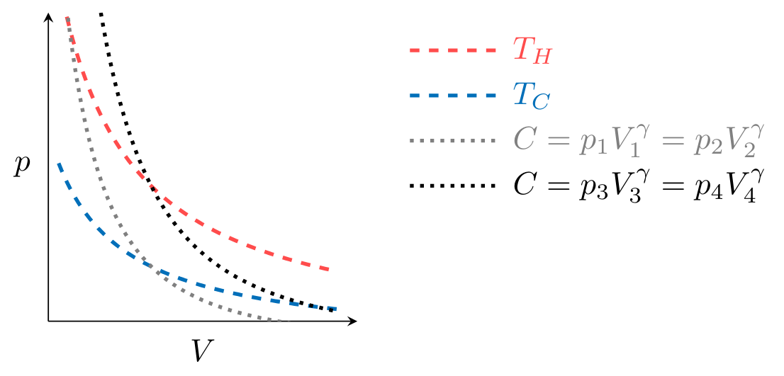
Figure 4: $pV$ curves for ideal gas expansion and compression in a Carnot cycle.

Processes $ 1 \to 2 $ and $ 3 \to 4 $ are adiabatic, meaning that during the process no heat transfer occurs. We will show later in the class that the adiabatic, reversible expansion or compression of an ideal gas must obey the relation

Ideal gas law in an adiabatic process #polytropic

$$ pV^{\gamma}=C $$

where $ \gamma $ and $ C $ are constants and $ \gamma > 1 $. Therefore these processes must fall on a curve defined by

Ideal gas law in an adiabatic process #Pexpression

$$ p(V)=\frac{C}{V^{\gamma}}, $$

illustrated for two values of $ C $ by the dash-dot lines in Fig. CarnotpV.

Combining the $ p(V) $ relations for the ideal gas expansion and compression with the directionality of the work shown in Figs. PVwork1 and PVwork2, we can plot a Carnot cycle for an ideal gas on a $ pV $ diagram as shown in Fig. CarnotpVcycle.

The work done by the cycle $ W $ is positive and equal to the shaded area in Fig. CarnotpVcycle, where the net work is described as the sum of the work done during each of the processes,

$$ W= W_{12} + W_{23} + W_{34} + W_{41} $$

Figure 5: A $pV$ diagram for an ideal gas undergoing a Carnot cycle as depicted in Fig. CarnotCycle.

Isothermal Processes

For isothermal processes $ 2 \to 3 $ and $ 4 \to 1 $ the work is determined by the $ p(V) $ relation in Eqn. IG_eos2 which yields

$$ W_{23} =mRT_H\ln\left(\frac{V_3}{V_2}\right) \,\,\text{ and }\,\, W_{41} = mRT_C\ln\left(\frac{V_1}{V_4}\right) $$

Because temperature is not changing and the fluid is an ideal gas, the change in internal energy for these processes is zero. An energy balance on the gas for each of these processes yields

$$ Q_{23} = Q_{H} = W_{23} = mRT_H\ln\left(\frac{V_3}{V_2}\right) $$

where $ Q_H $ refers to the heat transferred into the system from the hot reservoir and

$$ Q_{41} = - Q_{C} = W_{41} = mRT_C\ln\left(\frac{V_1}{V_4}\right) $$

where $ Q_C $ refers to the heat transferred from the system to the cold reservoir.

Adiabatic Processes

For adiabatic, reversible processes $ 1 \to 2 $ and $ 3 \to 4 $ the work is given by

$$ W_{12} = \int_{V_1}^{V_2} \frac{C_{12}}{V^{\gamma}} dV \text{ and } W_{34} = \int_{V_3}^{V_4} \frac{C_{34}}{V^{\gamma}} dV $$

which, when integrated yield

$$ \begin{gathered}W_{12} =\frac{-C_{12}}{\gamma-1}\left(\frac{1}{V_2^{\gamma-1}} - \frac{1}{V_1^{\gamma-1}}\right) \\\text{ and } \\ W_{34} = \frac{-C_{34}}{\gamma-1}\left(\frac{1}{V_4^{\gamma-1}} - \frac{1}{V_3^{\gamma-1}}\right) \end{gathered} $$

Multiplying both sides of the relation in Eqn. polytropic by $ 1/V^{\gamma-1} $ and using the resulting relation, $ pV = C/V^{\gamma-1} $, combined with the ideal gas equation of state, we can express the work in the adiabatic, reversible processes as

$$ W_{12} =\frac{mR(T_C - T_H)}{\gamma - 1} \,\,\text{ and }\,\, W_{34} = \frac{mR(T_H - T_C)}{\gamma - 1} $$

illustrating that the work in these two processes are equal in magnitude but opposite in sign.

It is interesting to determine the relationship between volume and temperature in the end states of processes $ 1 \to 2 $ and $ 3 \to 4 $ for the ideal gas. For an infinitesimal change in internal energy $ dU $ no heat flow occurs, but an infinitesimal amount of $ pV $ work is done, $ \delta W = p dV $. We write this infinitesimal form of the energy balance as

$$ d U = \cancelto{0}{\delta Q} - \delta W = -p dV $$

For an ideal gas, $ dU/dT = mc_v $ and $ p = mRT/V $ so that

$$ c_v dT = -\frac{RT}{V} dV $$

Separating the volume $ V $ and temperature $ T $ and integrating, between states $ 1 $ and $ 2 $ yields

$$ \int_{T_C}^{T_H} \frac{c_v}{RT} dT = \ln\left(\frac{V_1}{V_2}\right). $$

Integrating between states $ 4 $ and $ 3 $ yields

$$ \int_{T_C}^{T_H} \frac{c_v}{RT} dT = \ln\left(\frac{V_4}{V_3}\right). $$

The left hand side of both Eqns. VT12 and VT43 are equal so that

$$ \ln\left(\frac{V_1}{V_2}\right) = \ln\left(\frac{V_4}{V_3}\right). $$

or equivalently\sidenote $ \ln(x/y) = \ln x - \ln y $.

$$ \ln\left(\frac{V_1}{V_4}\right) = \ln\left(\frac{V_2}{V_3}\right). $$

Recalling the results from the energy balances on the isothermal processes (Eqns. QH and QC) we can show that the ratio of the heat influx $ Q_H $ to heat loss $ Q_C $ is

$$ \frac{Q_H}{Q_C} = \frac{T_H\ln\left(\frac{V_3}{V_2}\right) }{T_H\ln\left(\frac{V_4}{V_1}\right)} $$

Applying Eqn. V1234, which defines the relationship between the states before and after the adiabatic processes, we obtain

Heat-temperature relationship #HeatTemp

$$ \frac{Q_H}{Q_C} = \frac{T_H}{T_C} $$

for an ideal gas undergoing a Carnot cycle.

Internal Energy Balance of the System

The total change in the internal energy of the Carnot cycle $ \Delta U $ can alternately be determined by an energy balance on the cycle

$$ \begin{aligned}\Delta U&= Q - W \label{Ebalance} \\&= Q_H - Q_C - W_{12} - \underbrace{W_{23}}_{=Q_H} - \underbrace{W_{34}}_{=-W_{12}} - \underbrace{W_{41}}_{=-Q_C} \label{Ebaldetailed} \\&= 0\end{aligned} $$

Thus the Carnot cycle is consistent with the energy change for a cycle in general.

Thermal Efficiency

This Carnot cycle turns heat input $ Q_H $ into work output $ W $. The thermal efficiency $ \eta $ for such a heat engine is given by

Heat engine efficiency

$$ \eta = \frac{\text{net work output}}{\text{heat input}} = \frac{W}{Q_H} $$

Combining $ \Delta U = 0 $ for a cycle, the expression for the energy balance on the cycle (Eqns. Ebalance and Ebaldetailed), and the temperature-heat transfer relationship found in Eqn. HeatTemp yields

Heat engine efficiency in terms of temperature only

$$ \eta = \frac{Q_H - Q_C}{Q_H} = 1-\frac{T_C}{T_H}. $$

A Carnot cycle produces the maximum possible efficiency for any heat engine. The efficiency can only approach $ 1 $ (equivalent to 100\%) when either $ T_C \to 0 $ or $ T_H \to \infty $, neither of which is physically attainable.

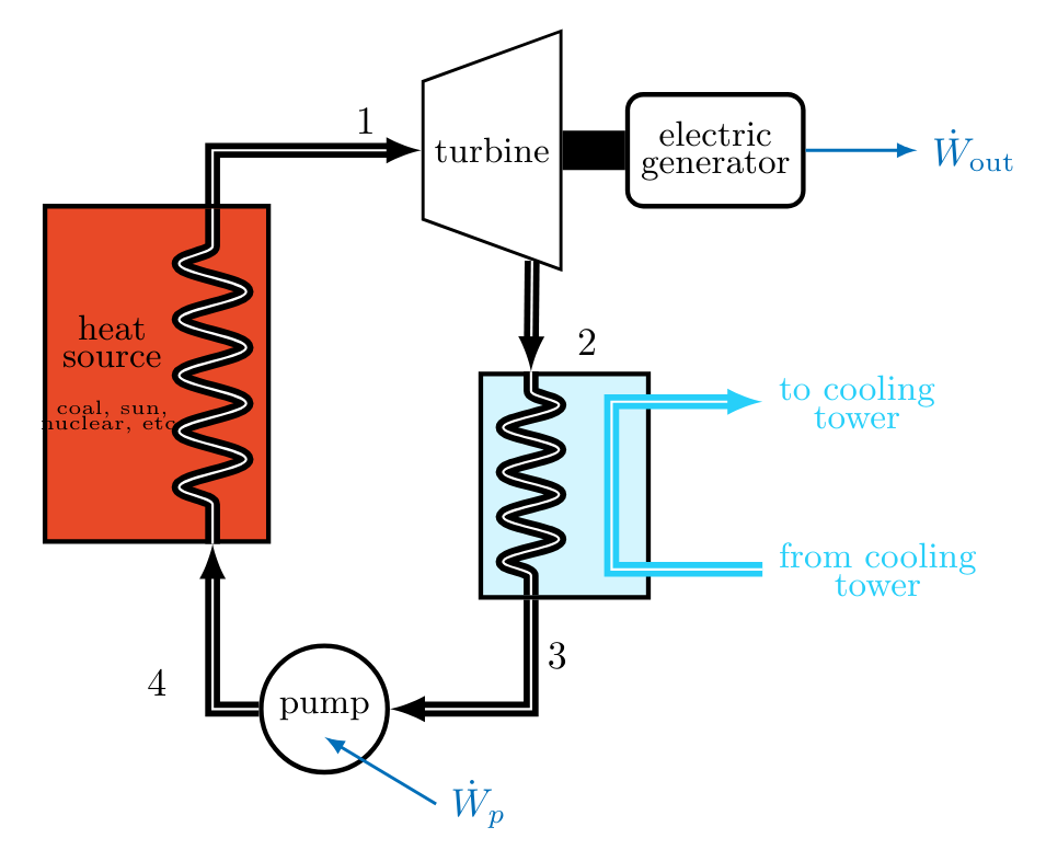
Figure 6: A schematic of a vapor power plant capable of undergoing a Rankine cycle.

Figure 7: A $T-s$ diagram of an ideal Rankine cycle.

A Rankine Cycle

The Rankine cycle is the basis for steam-electric power plants, which produce nearly 90% of all electricity worldwide. This cycle includes two isentropic processes, and utilizes isobaric heat transfers.

An ideal Rankine cycle consists of the following internally reversible processes:

Process $ 1\to 2 $ : Isentropic expansion of the working fluid through the turbine from saturated vapor at state $ 1 $ to the condenser pressure $ p_2 $.
Process $ 2\to 3 $ : Heat transfer from the working fluid as it flows at constant pressure $ p_2 = p_3 $ through the condenser, exiting as a saturated liquid at state $ 3 $.
Process $ 3\to 4 $ : Isentropic compression in the pump to state $ 4 $ in the compressed liquid region of the phase diagram.
Process $ 4\to 1 $ : Heat transfer to the working fluid as it flows at constant pressure $ p_4 = p_1 $ through the boiler to complete the cycle.

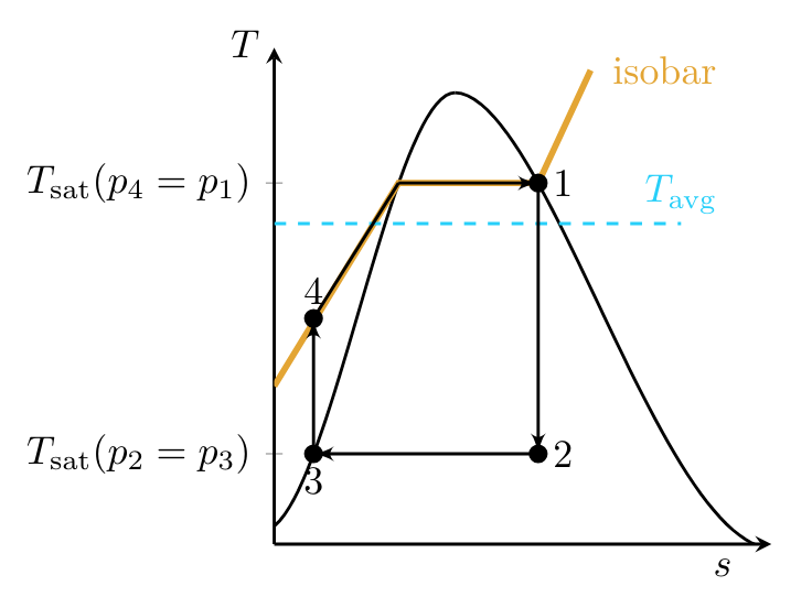
Instead, the condenser stream is taken to the saturated liquid state, so that only a compressed liquid must be pumped.\sidenote Cavitation is less of an issue in the two phase fluid used in the turbine since the vapor bubbles that form nearer the saturated vapor portion of the vapor dome are less driven to collapse. While state $ 4 $ could be taken all the way to $ T_{\text{sat}}(p_4 = p_1) $, this would also lead to practical difficulties since, to maintain an isothermal heat transfer, a large thermal reservoir would be required. Instead, the process from state $ 4 $ to state $ 1 $ follows an isobar as shown in the plot below.

For reversible processes, the second law can be written as:

Second law

$$ Q = \int T dS, $$

meaning that the area under the curve in a $ T $-$ s $ diagram corresponds to heat transferred to or from a system. Thus to approximate a Carnot cycle, an average temperature value at which the same heat transfer $ Q_H $ occurs can be approximated on the diagram.

Since the Carnot cycle tells us that the maximum thermal efficiency of a power cycle is:

$$ \eta = 1- Q_C/Q_H = 1-T_C/T_H $$

it is clear from Fig. TsDiagramRankine that a hypothetical Carnot cycle with maximum operating temperature $ T_H $ will always have a greater thermal efficiency than a Rankine cycle with the same maximum operating temperature since the average operating temperature of the Rankine cycle is lower.

Otto Cycle

The Otto cycle provides an approximation of the internal combustion engines that still make up the largest share of the transportation industry.

An automotive internal combustion engine uses a reciprocating piston-cylinder action to produce work. In a four-stroke engine

The intake valve is open and the piston makes an intake stroke to draw in a fresh charge, e.g., a combustible mixture of fuel and air.
The intake valve closes and the piston undergoes a compression stroke that increases the pressure and temperature of the air within. At the end of the compression, combustion is induced, e.g., via a spark plug.
A power stroke follows as the gas mixture expands, doing work on the piston.
Finally, the exhaust valve is opened and burned gases are purged during an exhaust stroke.

The Otto cycle simplifies this process by ignoring affects associated with the addition and removal of fuel. Instead it uses air, acting as an ideal gas, to provide insight into how such cycles can be optimized. The combustion itself is replaced by heat transfer and all processes are internally reversible. As a result, the Otto cycle consists of the following steps.

Process 1-2: Isentropic compression of the air as the piston moves from bottom to top.
Process 2-3: Constant-volume heat transfer to the air from an external source while the piston is at the top. (Approximates fuel ignition and rapid burning.)
Process 3-4: Isentropic expansion (power stroke).
Process 4-1: Constant-volume process in which heat is rejected from the air while the piston is at the bottom.

Note that because it is operating within a piston cylinder, the states the processes operate between are the state of the air in the closed piston cylinder system. This is different from the Rankine cycle, in which the stream states change by going through processes facilitated by different thermodynamics devices. We will show in class that the thermal efficiency of an Otto cycle can be expressed entirely as a function of the compression ratio, $ r $, defined as the ratio of the largest gas volume over the smallest $ V_1/V_2 $ according to:

Thermal efficiency of an Otto cycle

$$ \eta = 1-\frac{1}{r^{k-1}} $$

and shows that engine efficiency can be increased by inducing a larger change in piston chamber volume. Of course, further practical considerations, such as the increased weight of such an engine, provide other design constraints. We only touch on a few of these design constraints, but in general thermodynamics provides many of the key principles through which energy systems can be optimized.