Geometric properties
Center of mass (COM)
The total mass of a rigid body is as follows:
The center of mass of a rigid body can be calculated as follows:
Finding the center of mass allows us to treat complex shapes as point-masses with all their mass at the center of mass.
To find the center of mass of a body made up of composite shapes, we simply do the weighted average of each body by using the fact above.
Recap
| Type of shape | Operation |
|---|---|
| Simple shapes | Symmetry tables |
| Combination of simple shapes | Find each c.o.m and then combine |
| Complex shapes | Integrate |
Basic shapes
The centers of mass listed below are all computed directly from the integral #rcm-cm. Note the center of mass provided is the vector from point \(O\) (the reference origin).
Simplified shapes
The centers of mass listed below are all special cases of the basic shapes given in center of mass of basic shapes. Other special cases can be easily obtained by similar methods, or directly computing the integral.
Moment of inertia
The moment of inertia of a body, written \( I_{P,\hat{a}} \), is measured about a rotation axis through point \(P\) in direction \( \hat{a} \). The moment of inertia expresses how hard it is to produce an angular acceleration of the body about this axis. That is, a body with high moment of inertia resists angular acceleration, so if it is not rotating then it is hard to start a rotation, while if it is already rotating then it is hard to stop.
The moment of inertia plays the same role for rotational motion as the mass does for translational motion (a high-mass body resists is hard to start moving and hard to stop again).
Observe that the moment of inertia is proportional to the mass, so that doubling the mass of an object will also double its moment of inertia. In addition, the moment of inertia is proportional to the square of the size of the object, so that doubling every dimension of an object (height, width, etc) will cause it to have four times the moment of inertia.
Did you know?
We are always considering the moment of inertia to be a scalar value \( I \), which is valid for rotation about a fixed axis. For more complicated dynamics with tumbling motion about multiple axes simultaneously, it is necessary to consider the full 3 × 3 moment of inertia matrix:
The three scalar moments of inertia from #rem-ec appear on the diagonal. The off-diagonal terms are called the products of inertia and are given by
and similarly for the other terms. The angular momentum of a rigid body is given by \( \vec{H} = I \vec{\omega} \), which is the matrix product of the moment of inertia matrix with the angular velocity vector. This is important in advanced dynamics applications such as unbalanced rotating shafts and the precession of gyroscopes.
Parallel axis theorem
One consequence of the parallel axis theorem is that the moment of inertia can only increase as we move the rotation point \( P \) away from the center of mass \( C \). This means that the point with the lowest moment of inertia is always the center of mass itself.
A second consequence of the parallel axis theorem is that moving the point \( P \) along the direction \( \hat{a} \) doesn't change the moment of inertia, because the axis of rotation is not changing as the point moves along the axis itself.
Additive theorem
Basic shapes
The moments of inertia listed below are all computed directly from the integrals #rem-ec.
Simplified shapes
The moments of inertia listed below are all special cases of the basic shapes given in moment of inertia of basic shapes. Other special cases can be easily obtained by similar methods.
Summary: moment of inertia
| Mass moment of inertia (used in dynamics!) | Area moment of inertia | |||
|---|---|---|---|---|
| Other names | First moment of area | Second moment of area | Polar moment of area | |
| Description | Determines the torque needed to produce a desired angular rotation about an axis of rotation (resistance to rotation) | Determines the centroid of an area | Determines the moment needed to produce a desired curvature about an axis(resistance to bending) | Determines the torque needed to produce a desired twist a shaft or beam(resistance to torsion) |
| Equations | | | | |
| Units | \( \mathrm{mass} \ \mathrm{length} ^ 2 \) | \( \mathrm{length} ^ 3 \) | \( \mathrm{length} ^ 4 \) | \( \mathrm{length} ^ 4 \) |
| Typical Equations | | | | |
| Courses | Dynamics | Solid mechanics | Statics, solid mechanics | Solid mechanics |
Review?
Need a review of moment of inertia (second moment of area)?
This content has also been in statics.
The second moment of area determines the moment needed to produce a desired curvature about an axis (resistance to bending).
Instantaneous center (M)
- For a rigid body moving in 2D (rotating and possibly translating)
- Instantaneous center “M” is the point on or off the rigid body that has zero velocity at that instant (i.e. no translation at this point)
- Point that the body rotates about (at that instant in time)
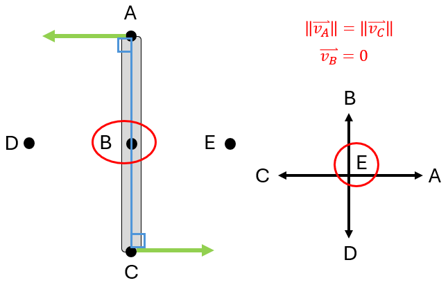
Graphical rules for finding M
(Assuming that figure is drawn to scale, including velocity vectors)
- Draw lines perpendicular to velocities
- If the lines intersect at a single point, that point is M
- If the lines are colinear:
- Draw 2 lines that connect the tips of velocity vectors
- If the lines intersect at a single point, that point is M
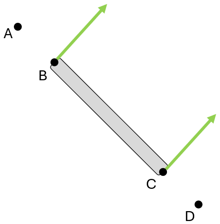
Find the instantaneous center (M) and the direction of \( \vec{v}_B \) of the beam.
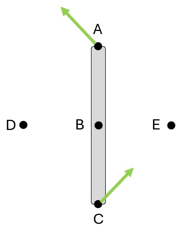
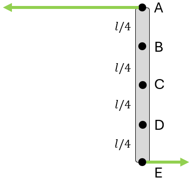
Find the instantaneous center (M) and the direction of \( \vec{v}_B \) of the beam.
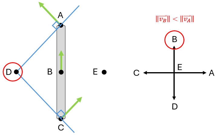
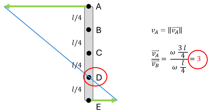
Find the instantaneous center (M) and the direction of \( v_A / v_B \) of the beam.
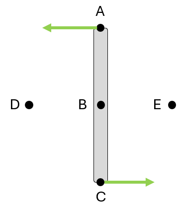
Find the instantaneous center (M).
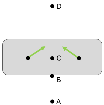
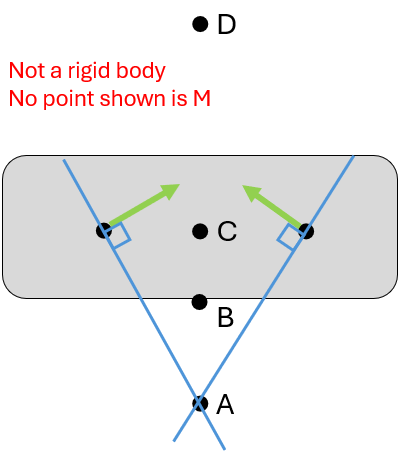
Find the instantaneous center (M).